From Vajra v0.4.1 to v0.5.0 to Rust backend: architecture notes and benchmark results

Update (Mar 4, 2026): A follow-up with vajra-search v0.2.1 build improvements and refreshed ZVec corpus-scale benchmarks is here: Vajra Search v0.2.1 update.

This post documents the technical continuity from:

1. Vajra lexical benchmarking work (BM25 engine comparisons),
2. Vajra vector search v0.4.1 and v0.5.0 in Python,
3. Rust-backed vajra_search HNSW with PyO3 bindings.

It focuses on engineering decisions and measured behavior, not language advocacy.

A detailed preprint version of this work is being prepared for arXiv submission.

The intended audience is engineers who care about retrieval systems in production: index build windows, latency envelopes, recall stability, and integration constraints.

1) Continuity: BM25 -> vector search -> Rust backend

flowchart LR
    A["Vajra BM25 benchmark phase\n(lexical IR)"] --> B["Vajra vector search v0.4.1\nPython + NumPy HNSW"]
    B --> C["Vajra vector search v0.5.0\nPython hot-path fixes"]
    C --> D["Vajra Rust backend\n`vajra_search` + PyO3"]

    A --> A1["Compared against\nBM25S, Tantivy, Pyserini"]
    C --> C1["Trigger: ZVec comparison\nshowed large build/query gaps"]
    D --> D1["Goal: preserve Python API\nmove ANN hot loops into Rust"]

2) Prior benchmark context (before vector v0.4.1)

Before the vector-search re-engineering, Vajra was benchmarked as a BM25 engine against multiple systems. The original technical report is here:

• Vajra BM25 benchmark and technical comparison report (original)

That report includes comparisons against:

• bm25s
• bm25s-parallel
• tantivy
• pyserini
• vajra-parallel

A compact snapshot from that phase:

This prior work matters because it established a benchmarking discipline used again for vector search: explicit baselines, fixed query protocol, and metric-level reporting.

That continuity matters because the Rust work should not be interpreted as a fresh benchmark starting point. It is a continuation of the same measurement practice and the same operational questions from the BM25 phase: what do we gain, what do we lose, and what trade-offs can be controlled explicitly.

3) ZVec as the trigger for v0.5.0 re-engineering

The initial Feb 22 baseline established the v0.4.1 gap against ZVec at 10k vectors.

• Re-engineering Vajra's vector search with inspiration from ZVec (baseline + deep profiling)

That same post contains the full v0.5.0 optimization walkthrough (six implementation fixes), which is the canonical source for the Python-side gains before Rust.

3.1 Baseline (v0.4.1)

3.2 Gains in v0.5.0 (from the separate profiling post)

Net effect from that stage:

• Build gap to ZVec reduced from roughly 207x to about 36x.
• Query gap to ZVec reduced from roughly 8.5x to about 1.6x.

At this stage, the engineering question changed from "can Python be optimized?" to "which remaining costs are structural and should move to a systems layer?"

4) Why move to Rust after v0.5.0

After v0.5.0, two constraints remained:

1. per-step interpreter overhead in HNSW hot loops,
2. mutable graph updates under heavy insertion/search workloads.

Rust was used to address those constraints while keeping the Python interface stable.

The design goal was not to replace the Python developer surface. The goal was to preserve the same API ergonomics while moving the high-frequency ANN primitives (graph traversal, candidate-heap mutation, distance dispatch) into a lower-overhead execution layer.

4.1 Architectural motivations

• Predictable memory behavior: contiguous vector storage and explicit layered adjacency reduce pointer-chasing variance in traversal-heavy loops.
• Lower hot-path overhead: candidate-heap updates and distance dispatch run in compiled code rather than Python-level dispatch.
• Safer mutation semantics: Rust ownership/borrowing constraints make graph-update paths easier to reason about under heavy insert/search cycles.
• Throughput headroom: batch query paths can use native parallel execution (Rayon) without changing the Python API.
• No API break for users: PyO3 keeps the Python entry points stable while delegating execution to Rust.

4.2 Python-Rust integration map

flowchart TB
    subgraph PY["Python surface"]
      P1["vajra_search.vector.NativeHNSWIndex"]
      P2["VajraVectorSearch / HybridSearchEngine"]
    end

    subgraph FFI["PyO3 / FFI boundary"]
      F1["PyHnswIndex\n(vajra-python/src/lib.rs)"]
    end

    subgraph RS["Rust core"]
      R1["HnswIndex\n(index.rs)"]
      R2["HnswGraph\n(graph.rs)"]
      R3["beam_search_fast + greedy_descent\n(search.rs)"]
      R4["Metric / distance kernels\n(distance.rs)"]
      R5["HnswNavigationCoalgebra\n(coalgebra.rs)"]
      R6["bincode persistence\n(save/load)"]
    end

    P2 --> P1 --> F1 --> R1
    R1 --> R2
    R1 --> R3
    R3 --> R4
    R5 -. "parity reference" .-> R3
    R1 --> R6

4.3 Custom HNSW implementation notes

The Rust HNSW implementation in crates/vajra-hnsw is not a wrapper around an external ANN library. It is implemented directly for this stack, including:

• graph storage (Vec<f32> vectors + layered adjacency),
• upper-layer greedy descent,
• layer-0 beam search (beam_search_fast),
• profile parameter surface (M, ef_construction, ef_search, use_heuristic),
• explicit coalgebra reference path for parity and verification.

In practice, this means benchmark deltas can be attributed to Vajra's implementation choices instead of hidden behavior in a third-party ANN binding.

5) Critical path differences: quality vs fast vs instant

Profiles are not just parameter presets; they change traversal work in both build and query paths.

M and ef_construction primarily shape insertion/build work (graph connectivity and candidate exploration), while ef_search shapes query-time frontier size. Disabling heuristics changes neighbor-selection cost and can materially reduce CPU work at some recall cost.

A practical operating pattern follows:

1. boot with instant for low startup latency,
2. rebuild asynchronously with quality,
3. atomically swap index handles when quality build completes.

This pattern should be read as an explicit control-plane design: startup latency and final recall are treated as separate objectives with a deterministic handoff.

5.1 Formalization: Profile-Lambda Retrieval Architecture (PLRA)

The deployment pattern above is structurally similar to Lambda Architecture in data engineering (Databricks glossary), but adapted for ANN index lifecycle rather than stream/batch ETL.

I refer to this as Profile-Lambda Retrieval Architecture (PLRA):

• Serving/Instant path: minimal-connectivity index for immediate availability.
• Speed/Fast path: moderate-cost index for better steady latency/recall while rebuilds continue.
• Batch/Quality path: high-recall full build in the background.
• Reconciliation: atomic index-handle swap when quality build is ready.

flowchart LR
    I["Instant profile
lowest startup cost"] --> S["Serve traffic immediately"]
    S --> F["Optional fast profile
moderate recall/cost"]
    S --> Q["Quality rebuild
high recall, higher build cost"]
    F --> Q
    Q --> A["Atomic swap to quality index"]

This gives a reproducible control surface: startup SLOs are decoupled from final ranking quality, and quality can be converged asynchronously.

Conceptually, PLRA is useful because it turns a tuning trade-off into an architecture primitive: profile transitions become part of deployment policy rather than ad-hoc runtime tweaking.

6) Current Rust benchmark snapshot (Wikipedia vectors)

Benchmarks were run for 1k, 10k, 20k, and 50k vectors.

6.1 Build/recall at 50k

6.2 Query at 50k

6.3 Figures

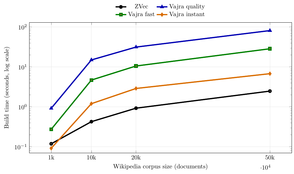
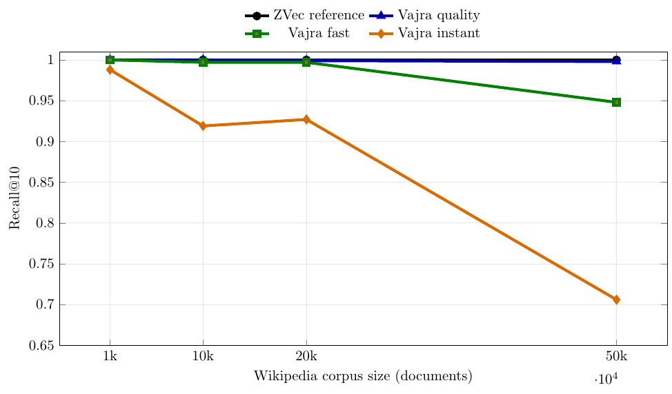
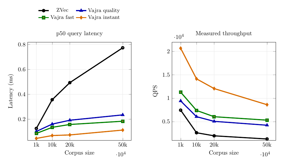
Reading these plots together:

• Build time separates profiles the most as corpus size grows.
• Query latency stays low for all Vajra profiles in this setup.
• Recall degradation is concentrated in instant, while quality remains close to the reference.
• fast acts as a middle operating point for teams that need lower build cost without dropping to instant recall.

7) Reproduction notes (Wikipedia data source)

The benchmark corpus slices are sourced from ir_benchmark_data, which is built from Wikipedia-focused IR corpora used in prior Vajra benchmarking.

At a high level:

1. Acquire documents from WikIR corpora through ir_datasets (for example wikir/en78k, with smaller fallback sets).
2. Normalize into JSONL snapshots with stable fields (id, title, content, metadata).
3. Generate embeddings (all-MiniLM-L6-v2, 384d) and keep the same embedding cache across engine/profile runs.

4. Slice consistently into 1k/10k/20k/50k subsets for direct comparisons.

5. Data location used locally: ~/Github/ir_benchmark_data

6. Benchmark harness location: ~/Github/zvec_vajra_benchmark

Detailed reproducibility instructions (including expected directory wiring and commands) are provided in:

• vajra_search_engine/reproduction.md

8) References

• Vajra BM25 benchmark and technical comparison report (original)
• Vajra BM25 architecture post (Dec 24, 2025)
• Vajra vector search v0.4.1 -> v0.5.0 engineering post (Feb 22, 2026)
• Databricks: Lambda Architecture
• ZVec