Jorge Luis Borges' short story "Tlön, Uqbar, Orbis Tertius" describes a fictional world where the inhabitants speak a language with no nouns - only verbs. There are no objects, only processes. The moon rising over water is not a thing acting upon another thing; it is a single verb, a happening. Below is the page from Borges' aforementioned story that inspired this line of thinking.

This idea was lodged in my mind for years. What if we took it seriously? What if we built a mathematical framework where processes are primitive and objects emerge as stable patterns? The philosophical implications of this seemed enormous, each time I thought about it. Every cell in the human body has an expiration date, but the human body itself maintains its rough shape over time. We experience the process of aging. Turbulence transforms the way molecules of water behave, as they leave the outlet of a tap and drop down; we see laminar flow transition to turbulent flow. Double pendulums behave in very unpredictable ways even if we repeat experiments with them from just mildly different initial conditions, and at the same time, grand phenomena such as the Great Red Spot on Jupiter are stable and predictable for years. The moon's orbit around the Earth seems a stable process but over millennia, there are minor variations in the orbits of all celestial bodies. You get the idea - the list of phenomena that could be characterised as emergent are endless and all around us.
What I have been exploring with Tlon mathematics is the possibility that we could describe many of these emergent phenomena, or even phenomena we consider rule-based, or stable, from the lens of a process-first mathematical paradigm. I'd learned some category theory basics earlier in the year, and wanted to see if I could build an algebra that addressed just such a process-centric approach to systems modelling. Later in the year, with Claude Code as my collaborator, I finally attempted to build the scaffolding, proofs, and the "house" on top of which actual mathematical systems and conjectures could be posited.
The result of all this rumination and exploration with Claude Code is Tlön Mathematics. I will interchangeably use Tlön and Tlon, for the convenience of typing is an important aspect of the process of communication. Tlön (Tlon) mathematics is a mathematical framework built on top of 20 axioms across 6 groups, with theorems, proofs, and concrete implementations in Python that convert the mathematical foundation into a computational foundation that demonstrates the concepts through various systems simulations, including simulations of dynamical systems. As a purely intellectual exercise, this was quite satisfying, because, well, a set of core axioms was converted through sequential rules into a whole mathematical world view, and one inspired by a work of fiction, by one of my favourite authors, at that. Working with the ideas of Tlon mathematics has made me appreciate how we can frame dynamical systems and the emergence of objects in the physical world in a different way.
The Central Inversion
In conventional mathematics, objects exist first and processes act upon them. A rock exists; erosion happens to it. A planet exists; orbital motion happens to it.
Tlön inverts this, in a specific way: processes are fundamental, and objects are stable patterns - processes that maintain themselves through repetition. This isn't to say that Tlon mathematics bypasses the established rules of mathematics, and to the contrary, Tlon mathematics is built on top of a category theoretic structure, like other algebras. Identities, relationships like associativity and the like can be proven in this system of mathematics like in others.
As I described in examples above, objects are our default mode of viewing and understanding the world around us, and Tlon challenges this convention, based on the phenomena that we do see that indicate how this object-property-interaction ontology in our heads cannot explain transient objects or objects like the Mandelbrot set. Through the lens of Tlon, therefore, a rock isn't an object, but the result of a stable process that has produced an aggregation of things that appears to be a rock, and that we can classify as such. The rock's changes over time, be it erosion through wind or rain or other phenomena, and these processes that give the rock its characteristics are also processes. A planet is a specific aggregation of matter that has emerged as a stable process (or a large set of stable processes), resulting in the object we see as the planet. While this may seem like splitting hairs when we write it down in English, it becomes much clearer when we write it down in terms of definitions, assertions we have as axioms, and allow the system of mathematics to guide us in terms of the properties that emerge as a consequence of these foundations. Tlon serves as a mathematical scaffolding for discussing processes whose physics have been established, and as a process algebra, but perhaps does not serve as a physics scaffolding, and I have a hunch that this is something I will discover in time as I work with Tlon mathematics.
How Objects Emerge from Processes
The key insight is formal: an object in Tlon is defined as an equivalence class of stable processes:
A process is stable when repeating it is equivalent to doing it once:
This definition inverts traditional ontology:
| Traditional View | Tlon View |
|---|---|
| Objects exist primitively | Processes exist primitively |
| Processes act on objects | Objects emerge from stable processes |
| "What things exist?" | "Which processes are stable?" |
Concrete examples:
- Flame: The combustion process $\pi_{\text{flame}}$ is stable; sustained burning is equivalent to momentary burning in terms of the pattern. The "flame" we perceive is the equivalence class $[\pi_{\text{flame}}]$.
- Sorted array: The sorting process satisfies $\text{sort} ; \text{sort} \approx \text{sort}$. A sorted array is the stable fixed point.
- Planetary orbit: One complete orbit $\pi_{\text{orbit}}$ satisfies $\pi_{\text{orbit}} ; \pi_{\text{orbit}} \approx \pi_{\text{orbit}}$. The "orbit" is the stable pattern, not the planet.
- Standing wave: Two traveling waves interfere to produce a pattern that maintains itself through time.
In each case, the "object" is not a thing but a self-sustaining pattern of activity. The question "what objects exist?" becomes an algebraic question: "which processes are idempotent under sequential composition?"
Tlon's processes and stability
Tlon could potentially allow us to model phenomena around us in dynamic slices. For example, a planet need not be modelled as an object that has a certain range of motions owing to fundamental forces such as gravity, but it could be modelled in Tlon terms as an orbital process that is stable, resulting in accretion and the the object we see as the planet. Geophysical phenomena may be similarly modeled starting from the processes we observe.
Stability is defined as follows:
A stable process is one where a repetition of the process is equivalent to performing it once. In algebra, such elements are called idempotent. These are the closest thing to "objects" in Tlön - self-maintaining patterns that persist through repetition.
The 20 Axioms
The framework is built on 20 axioms organized into 6 groups:
| Group | Axioms | What They Establish |
|---|---|---|
| A | A1-A2 | Existence: Processes exist and have duration |
| B | B1-B4 | Sequential composition. We introduce the $;$ operator "then" |
| C | C1-C5 | Concurrent composition ($\parallel$): "while" |
| D | D1-D5 | Interference: How concurrent processes affect each other |
| E | E1-E2 | Stability: Idempotent processes as "objects" |
| F | F1-F4 | Equivalence: Behavioral interchangeability |
Complete Axiom List
Group A: Existence
- A1: $\exists\pi$ (Process($\pi$)) — Processes exist
- A2: $\exists!\varepsilon$ $(|\varepsilon| = 0)$ — Unique null process with zero duration
Group B: Sequential Composition
- B1: $\forall\pi,\rho \Rightarrow \text{Process}(\pi ; \rho)$ — Closure
- B2: $(\pi ; \rho) ; \sigma \approx \pi ; (\rho ; \sigma)$ — Associativity
- B3: $\pi ; \varepsilon \approx \pi \approx \varepsilon ; \pi$ — Identity
- B4: $|\pi ; \rho| = |\pi| + |\rho|$ — Duration additivity
Group C: Concurrent Composition
- C1: $\forall\pi,\rho \Rightarrow \text{Process}(\pi \parallel \rho)$ — Closure
- C2: $(\pi \parallel \rho) \parallel \sigma \approx \pi \parallel (\rho \parallel \sigma)$ — Associativity
- C3: $\pi \parallel \rho \approx \rho \parallel \pi$ — Commutativity
- C4: $\pi \parallel \varepsilon \approx \pi$ — Identity
- C5: $|\pi \parallel \rho| = \max(|\pi|, |\rho|)$ — Duration maximum
Group D: Interference
- D1: $\text{Int}(\pi, \rho) \approx \text{Int}(\rho, \pi)$ — Symmetry
- D2: $\text{Int}(\pi, \pi) \approx \pi$ — Self-interference
- D3: $\text{Int}(\pi, \varepsilon) \approx \pi$ — Null non-interference
- D4: $|\pi| = |\rho| \Rightarrow \pi \parallel \rho \approx \pi ; \text{Int}(\pi, \rho) ; \rho$ — Decomposition
- D5: $\pi \approx \pi' \land \rho \approx \rho' \Rightarrow \text{Int}(\pi, \rho) \approx \text{Int}(\pi', \rho')$ — Congruence
Group E: Stability
- E1: $\text{Stable}(\pi) \Leftrightarrow \pi ; \pi \approx \pi$ — Idempotence definition
- E2: $\exists\pi$ $(\text{Stable}(\pi) \land \pi \not\approx \varepsilon)$ — Non-trivial stability exists
Group F: Equivalence
- F1: $\pi \approx \pi$ — Reflexivity
- F2: $\pi \approx \rho \Rightarrow \rho \approx \pi$ — Symmetry
- F3: $\pi \approx \rho \land \rho \approx \sigma \Rightarrow \pi \approx \sigma$ — Transitivity
- F4: $\approx$ respects $;$ and $\parallel$ — Congruence
Three axioms deserve particular attention:
Axiom E1 (Stability Definition):
A process is stable if repeating it yields the same thing. The null process $\varepsilon$ (doing nothing) is trivially stable. But other stable processes exist too; these are the emergent "objects", the results of stability.
Axiom B4 (Duration Additivity):
Sequential composition adds durations. If a process $\pi$ has a duration of 3 units and another $\rho$ has a duration of 5 units, doing them in sequence takes 8 units. This is self-evident and agrees with common algebras we are familiar with.
Axiom C2 (Concurrent Commutativity):
Unlike sequence (where order matters), concurrence is symmetric. "$\pi$ while $\rho$" is the same as "$\rho$ while $\pi$."
Key Theorems
From these axioms, several important results follow. We validate the following Tlon theorems using a category theory foundation, which becomes necessary as the latter is a scaffolding for many mathematical systems.
Theorem 1.1: Sequential composition forms a monoid - $(\text{Process}, ;, \varepsilon)$ has closure, associativity, and identity. Here ; represents the sequential composition operator, and $\varepsilon$ represents the null process.
Proof: Closure by B1, associativity by B2, identity by B3. ∎
Theorem 1.2: Concurrent composition forms a commutative monoid - $(\text{Process}, \parallel, \varepsilon)$ additionally has commutativity. Here $\parallel$ represents the concurrent composition operator, and $\varepsilon$ represents the null process.
Proof: Closure by C1, associativity by C2, commutativity by C3, identity by C4. ∎
Theorem 4.3 (Power Collapse): If some process $\pi$ is stable, then $\pi^n \approx \pi$ for all $n \geq 1$. Sequential powers collapse for stable processes. Here $\approx$ represents the equivalence operator.
Proof: By induction. Base: $\pi^1 = \pi$. Step: If $\pi^n \approx \pi$, then $\pi^{n+1} = \pi^n ; \pi \approx \pi ; \pi \approx \pi$ (by stability). ∎
The Emergence Theorem: In any finitely-generated process space with non-trivial stable processes, the property "non-trivially stable" is emergent - it doesn't hold for any generator but must hold for some composite process.
Proof: See Tlon Theory Booklet, Theorem E1. The proof uses the level function $L(\pi)$ measuring compositional complexity. ∎
The Emergence Theorems
Tlon's approach to emergence is mathematically precise: it shows how stable patterns (objects, structures, dynamics) arise out of the interactions and compositions of unstable, transient parts. The theorems, drawn from the Tlon Theory Booklet, clarify different faces of emergence:
E2: Resonance Generates Emergent Stability
Theorem (Resonance Emergence):
If $\pi$ and $\rho$ are both unstable, but $\text{Stable}(\pi \parallel \rho)$, then stability is an emergent property of their combination.
Proof: By assumption, $\text{Stable}(\pi) = \text{false}$ and $\text{Stable}(\rho) = \text{false}$, yet $\text{Stable}(\pi \parallel \rho) = \text{true}$. The whole has a property neither part possesses. ∎
- Interpretation: Two chaotic or transient processes, when run concurrently, may form a composite process that is stable, even though neither is stable alone. This is resonance: the "whole is more than the sum of its parts" in a formal algebraic sense.
- Concrete Example:
In the Lotka-Volterra predator-prey model (Volterra, 1926; Lotka, 1925), the isolated prey or predator populations are unstable. But together, their interaction stabilizes the entire ecosystem into periodic cycles. A stable process emerges from their interplay.
E3: Objecthood is Emergent
Theorem (Emergence of Objects):
Non-trivial objects (i.e., equivalence classes of stable processes other than the null process) cannot exist at the primitive level. They arise only through composition and stabilization.
Proof: Objects are equivalence classes of stable processes. At level 0, only generators exist. Since non-trivial stability requires composition (by E1), objects first appear at level ≥ 1. ∎
- Interpretation:
In Tlon, objects are not presupposed. There are no building blocks waiting to be labeled as "objects"; instead, objects emerge from the closure and stabilization of processes. The question is not "what objects are there?" but "which processes are stable?" The stable patterns themselves are the objects.
E4: Downward Constraint (Emergent Constraint)
Theorem (Downward Constraint):
If $\pi = \sigma ; \tau$ is stable, then $\sigma ; \tau ; \sigma ; \tau \approx \sigma ; \tau$. The global stability of the composite process constrains the behaviors of its components.
Proof: If $\pi = \sigma ; \tau$ is stable, then $\pi ; \pi \approx \pi$ by E1. Substituting: $(\sigma ; \tau) ; (\sigma ; \tau) \approx \sigma ; \tau$. ∎
- Interpretation:
Emergent stability at a higher level (the composite process) imposes algebraic constraints on the lower-level sequences that compose it. This expresses a formal version of "downward causation": the stability of the whole feeds back to restrict the ways its parts can behave.
The full formal statements, proofs, and examples are presented in the Tlon Theory Booklet.
The Doctrine of No Inverses
One of the most striking results is that process inverses are ontologically forbidden. For any process $\pi$ with positive duration, there exists no process $\rho$ such that $\pi ; \rho \approx \varepsilon$.
The argument is straightforward:
1. By Duration Additivity: $|\pi ; \rho| = |\pi| + |\rho| \geq |\pi| > 0$
2. But $|\varepsilon| = 0$
3. Therefore $\pi ; \rho$ cannot equal $\varepsilon$
Happenings cannot un-happen. The arrow of time is woven into the fabric of process composition. This is not a bug but a feature - it captures something fundamental about causality and time.
The correct concept is reversal, not inverse. A reversal $\rho$ of $\pi$ completes a stable cycle: $\text{Stable}(\pi ; \rho)$. The pendulum swings left ($\pi$), then right ($\rho$). The composite $\pi ; \rho$ is one complete oscillation - a stable process. Time passed; something happened. But the pattern is closed, self-sustaining.
The Code Structure
The mathematical scaffolding I've built for Tlon is also being represented in code, as a Python code base. I am perhaps undecided on whether this should be written in a functional programming language, which seems to provide first class abstractions to deal with the nuts and bolts of Tlon mathematics. In any case, the Python implementation has been helpful to simulate different kinds of systems and understand them with the scaffolding of Tlon mathematics.
The framework is implemented in Python with type hints and comprehensive tests. The core abstractions live in tlon/core/:
class Process(ABC):
    """Abstract base class for all processes."""

    @property
    @abstractmethod
    def duration(self) -> float:
        """Intrinsic temporal extent of the process."""
        pass

    def is_stable(self, tolerance: float = 1e-9) -> bool:
        """Axiom E1: Stable(π) ⟺ π ; π ≈ π"""
        return (self @ self).equiv(self, tolerance)

    def __matmul__(self, other):
        """Sequential composition: π @ ρ (represents π ; ρ)"""
        ...

    def __or__(self, other):
        """Concurrent composition: π | ρ (represents π ∥ ρ)"""
        ...
A number of concrete classes and patterns are implemented in the Tlon math codebase to make the abstract foundations operational and testable. Some illustrative examples:
class Sequence(Process):
    """A process representing a fixed sequence of sub-processes."""

    def __init__(self, steps: list[Process]):
        self.steps = steps

    @property
    def duration(self) -> float:
        return sum(s.duration for s in self.steps)

    def __matmul__(self, other: "Process") -> "Sequence":
        return Sequence(self.steps + ([other] if isinstance(other, Process) else list(other.steps)))

    def __or__(self, other: "Process") -> "Concurrent":
        return Concurrent([self, other])

    def equiv(self, other, tolerance=1e-9) -> bool:
        # Equivalence up to minor perturbations
        return (
            isinstance(other, Sequence) and
            len(self.steps) == len(other.steps) and
            all(s1.equiv(s2, tolerance) for s1, s2 in zip(self.steps, other.steps))
        )
A Concurrent class expresses parallel composition:
class Concurrent(Process):
    """Represents concurrent execution of several processes."""

    def __init__(self, parts: list[Process]):
        self.parts = parts

    @property
    def duration(self) -> float:
        return max(p.duration for p in self.parts) if self.parts else 0.0

    def __matmul__(self, other: "Process") -> "Sequence":
        return Sequence([self, other])

    def __or__(self, other: "Process") -> "Concurrent":
        return Concurrent(self.parts + ([other] if isinstance(other, Process) else list(other.parts)))

    def equiv(self, other, tolerance=1e-9) -> bool:
        # Permutation-insensitive equivalence
        return (isinstance(other, Concurrent) and
                set(self.parts) == set(other.parts))
Single-shot atomic happenings like events are provided by primitives:
class Event(Process):
    """An instantaneous process (duration == epsilon > 0)."""

    def __init__(self, label: str, duration: float = 1e-6):
        self.label = label
        self._duration = duration

    @property
    def duration(self) -> float:
        return self._duration

    def __matmul__(self, other: "Process"):
        return Sequence([self, other])

    def __or__(self, other: "Process"):
        return Concurrent([self, other])

    def equiv(self, other, tolerance=1e-9) -> bool:
        return (
            isinstance(other, Event) and
            self.label == other.label and
            abs(self.duration - other.duration) < tolerance
        )
Oscillation can be implemented for resonance experiments:
class Oscillation(Process):
    """Models periodic processes (e.g., Lotka-Volterra cycles, pendulum)."""

    def __init__(self, period: float, cycles: int = 1):
        self.period = period
        self.cycles = cycles

    @property
    def duration(self) -> float:
        return self.period * self.cycles

    def __matmul__(self, other: "Process"):
        # Concatenating oscillatory cycles
        if isinstance(other, Oscillation) and other.period == self.period:
            return Oscillation(self.period, self.cycles + other.cycles)
        return Sequence([self, other])

    def __or__(self, other: "Process"):
        return Concurrent([self, other])

    def equiv(self, other, tolerance=1e-9) -> bool:
        return (
            isinstance(other, Oscillation)
            and abs(self.period - other.period) < tolerance
            and self.cycles == other.cycles
        )
These classes allow modeling of concrete systems:
- A NBodyOrbit class (not shown here) composes body-body pairwise processes.
- DampedOscillator for irreversible transients (energy dissipation).
- StableEquilibrium for fixed points.
- Reversal for stable cycles, e.g., as Oscillation(period=T, cycles=1).
The abstraction boundary: any process that satisfies is_stable() according to the abstract axioms above will behave as a "Tlön object": its composition is idempotent (up to tolerance), making mathematical stability operational in code.
Processes are classified in a purity spectrum:
| Class | Sequentially Stable | Concurrently Stable | Example |
|---|---|---|---|
| Transient | No | No | Double pendulum (chaotic) |
| Seq. Stable | Yes | No | Kepler orbits |
| Conc. Stable | No | Yes | Individual oscillators |
| Pure | Yes | Yes | Fixed points, equilibria |
From Primitives to Simulations
The abstract Process class needs to model actual dynamical systems to be useful. The DynamicalProcess base class bridges Tlon's axioms to numerical simulation:
class DynamicalProcess(Process):
    """
    Base class for dynamical system processes.

    A trajectory segment (x₀ → x₁ over dt) is a process.

    Mapping to Tlon axioms:
        - Duration = time interval of evolution
        - Sequential (;) = concatenate trajectories
        - Concurrent (∥) = parallel systems (with coupling)
        - Stability = fixed points / limit cycles
        - Interference = coupling between systems
    """

    def _seq_compose(self, other: 'DynamicalProcess') -> 'DynamicalProcess':
        """Sequential: evolve self, then continue from self's final state."""
        continued = other._evolve(self.final_state, other.duration)
        return self._make_process(TrajectorySegment(
            initial_state=self.initial_state,
            final_state=continued.final_state,
            dt=self.duration + other.duration,  # Axiom B4
        ))

    def _conc_compose(self, other: 'DynamicalProcess') -> 'DynamicalProcess':
        """Concurrent: run both systems in parallel."""
        max_dt = max(self.duration, other.duration)  # Axiom C5
        # Create product system...
This pattern allows any ODE system to be wrapped as a Tlon process. The framework handles composition, stability checking, and equivalence. The subclass provides the vector field.
Simulations: Seeing Tlön in Action
Implementing dynamical systems and watching them demonstrate Tlön concepts has been where the framework proves itself. The Tlon framework provides three things that standard numerical integration does not: a consistent API for composition, automatic stability checking, and a vocabulary for classifying dynamical behavior.
The Double Pendulum: Transient Processes
The double pendulum is the canonical example of chaos in classical mechanics (Strogatz, 2015). In Tlön terms, it demonstrates transient processes - trajectories that never return to themselves.
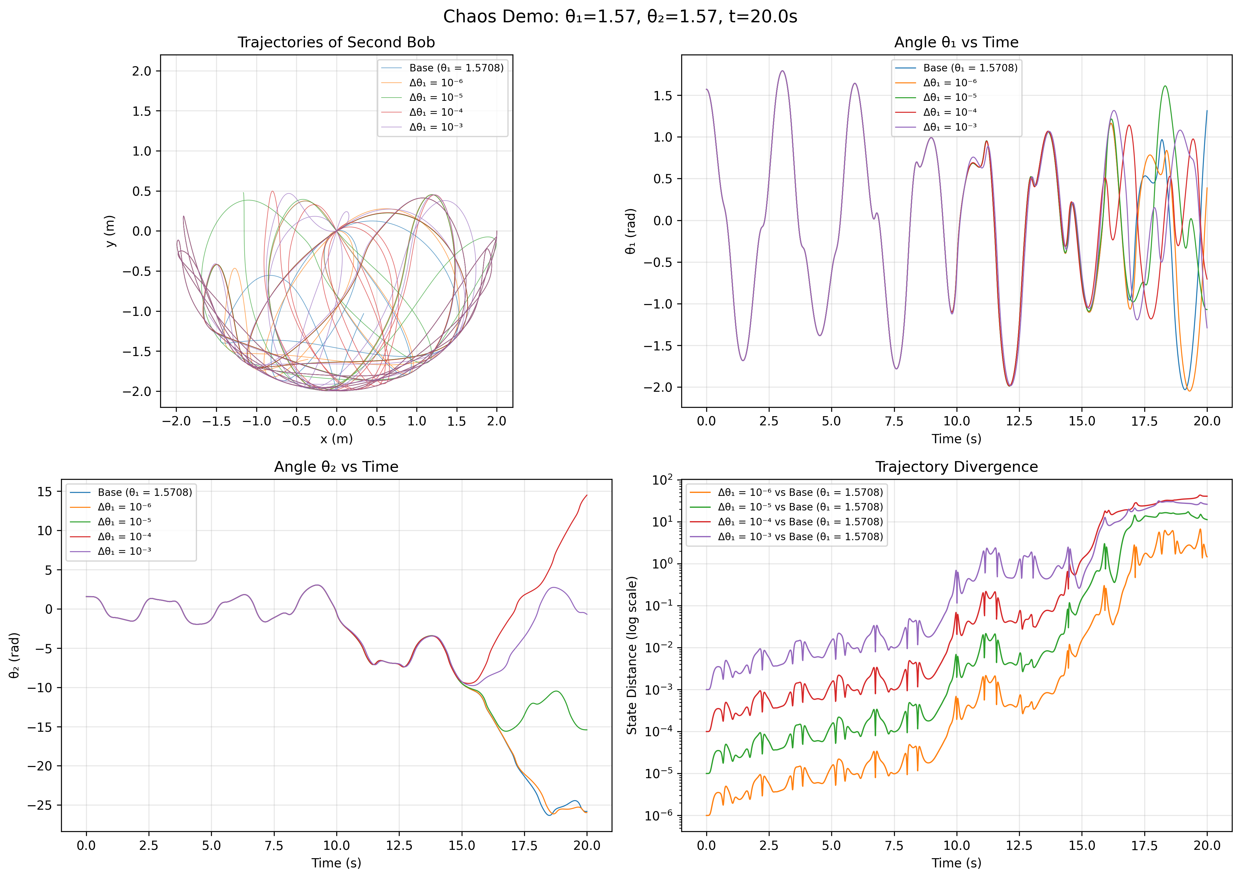
Two double pendulums started with nearly identical initial conditions ($10^{-6}$ difference). Within seconds, they diverge completely. This is the signature of a transient process.
The implementation wraps the Lagrangian equations of motion in the Tlon Process interface:
class DoublePendulumProcess(Process):
    """
    A double pendulum trajectory as a Tlon Process.

    Tlon interpretation:
        - Process = trajectory segment (x₀ → x₁ over dt)
        - Duration = time elapsed
        - Sequential (;) = concatenate trajectories
        - Stability = fixed points (equilibria)
        - Equivalence = same final state (behavioral)
    """

    def _derivatives(self, state: NDArray) -> NDArray:
        """Lagrangian equations: d/dt [θ1, θ2, ω1, ω2]"""
        θ1, θ2, ω1, ω2 = state
        Δθ = θ1 - θ2
        denom = 2 * m1 + m2 - m2 * np.cos(2 * Δθ)

        # Angular accelerations from Euler-Lagrange equations
        α1 = (-g * (2*m1 + m2) * np.sin(θ1) - m2*g*np.sin(θ1 - 2*θ2)
              - 2*np.sin(Δθ) * m2 * (ω2**2*L2 + ω1**2*L1*np.cos(Δθ))) / (L1 * denom)
        α2 = (2*np.sin(Δθ) * (ω1**2*L1*(m1+m2) + g*(m1+m2)*np.cos(θ1)
              + ω2**2*L2*m2*np.cos(Δθ))) / (L2 * denom)

        return np.array([ω1, ω2, α1, α2])

    def _seq_compose(self, other: 'DoublePendulumProcess') -> 'DoublePendulumProcess':
        """Sequential: continue evolution from self.final_state."""
        final, traj, times = self._integrate_rk4(self._final, other.duration)
        return DoublePendulumProcess(
            initial_state=self._initial,
            final_state=final,
            dt=self._dt + other.duration,  # Axiom B4: durations add
        )

    def equiv(self, other: 'Process', tolerance: float = 1e-6) -> bool:
        """Behavioral equivalence: same final state."""
        if not isinstance(other, DoublePendulumProcess):
            return False
        return self._final.distance_to(other._final) < tolerance
The Process interface forces you to think about what "composing" trajectories means: sequential composition concatenates them, and the duration axiom (B4) ensures time accounting is correct. The stability methods provide immediate feedback about the system's character:
# Create and evolve from a chaotic initial condition
initial = PendulumState(theta1=np.pi/2, theta2=np.pi/2, omega1=0, omega2=0)
proc = DoublePendulumProcess.evolve(initial, dt=10.0)

# The framework answers: is this stable?
print(proc.is_stable())           # False - never returns to itself
print(proc.purity_class())        # "transient"

# Sequential composition: what happens if we run it twice?
proc_twice = proc @ proc  # π ; π
print(proc_twice.equiv(proc))     # False - chaos means π;π ≉ π

# Perturb and compare: sensitivity to initial conditions
perturbed = PendulumState(theta1=np.pi/2 + 1e-6, theta2=np.pi/2, omega1=0, omega2=0)
proc_perturbed = DoublePendulumProcess.evolve(perturbed, dt=10.0)
print(f"Divergence: {proc._final.distance_to(proc_perturbed._final):.2f}")  # Large!
Tlon mathematics makes the transience of the double pendulum operational. You do not just observe that trajectories diverge; you ask the algebraic question "is $\pi ; \pi \approx \pi$?" and get a definitive answer. The double pendulum fails the stability axiom, and this failure is the formal definition of chaos in the Tlon framework.
The N-Body Problem: Stability is Special
This simulation provides the purest illustration of the Tlön principle: stability is special, not generic. The N-body problem is one of the oldest in classical mechanics; Poincaré's work on it (Poincaré, 1890) in the early 1900s founded the entire field of dynamical systems.

The transition from order to chaos: two-body orbits are stable and predictable, while three or more bodies exhibit chaotic trajectories.
The Tlon framework makes the comparison between $N=2$ and $N=3$ crisp:
# Two-body system: circular orbit
two_body = NBodyState.two_body_circular(m1=1.0, m2=1.0, separation=1.0)
proc_2 = NBodyProcess.evolve(two_body, dt=15.0)

# Three-body system: Pythagorean configuration (3-4-5 triangle)
three_body = NBodyState.three_body_pythagorean()
proc_3 = NBodyProcess.evolve(three_body, dt=15.0)

# The framework provides stability analysis methods
print(f"Two-body Lyapunov estimate:   {proc_2.lyapunov_estimate():.4f}")   # ~0.3
print(f"Three-body Lyapunov estimate: {proc_3.lyapunov_estimate():.4f}")   # ~1.1

print(f"Two-body periodic stable:   {proc_2.is_periodic_stable()}")  # True
print(f"Three-body periodic stable: {proc_3.is_periodic_stable()}")  # False
Two-body problem ($N=2$): Integrable, stable. The system reduces to Kepler orbits with two conserved quantities (energy, angular momentum). Trajectories form clean, closed paths. Lyapunov exponent $\sim 0.3$.
Three-body problem ($N \geq 3$): Generically chaotic, transient. Not enough conserved quantities to constrain the motion. Trajectories are erratic and unpredictable. Lyapunov exponent $\sim 1.1$ (3-4x more chaotic).
There are exceptions - the famous figure-8 orbit (Moore, 1993; Chenciner & Montgomery, 2000) shows that stability is possible for $N=3$, but only for measure-zero sets of initial conditions.
The Figure-8 Orbit: Stability Emerging from Chaos
The figure-8 orbit is remarkable: three equal masses chase each other around a figure-8 shaped path, each body following exactly the same trajectory but phase-shifted in time. It was discovered by Cris Moore (Moore, 1993) after searching systematically through initial conditions.
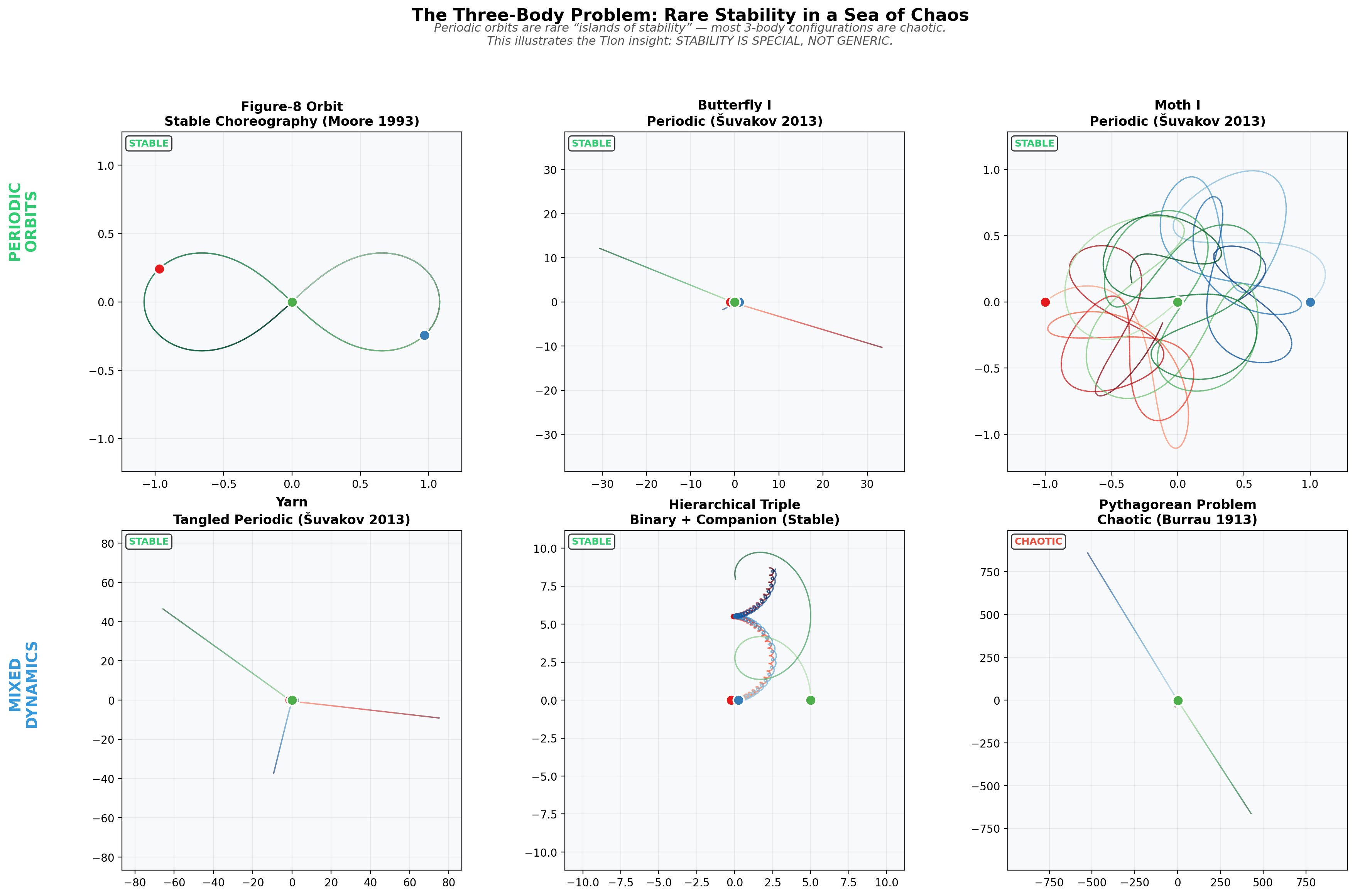
Six different three-body configurations: the figure-8 (top left) is the most famous stable choreography. Butterfly and Moth orbits (top middle, right) are more complex but still periodic. The Pythagorean configuration (bottom right) shows generic chaotic behavior.
Finding and verifying the figure-8:
# Create the figure-8 initial conditions
# Three equal masses at specific positions and velocities
figure8 = NBodyState.three_body_figure_eight()

print("Initial configuration:")
for i, body in enumerate(figure8.bodies):
    print(f"  Body {i+1}: pos=({body.x:.4f}, {body.y:.4f}), "
          f"vel=({body.vx:.4f}, {body.vy:.4f})")

# Initial configuration:
#   Body 1: pos=(-0.9700, 0.2431), vel=(0.4662, 0.4324)
#   Body 2: pos=(0.9700, -0.2431), vel=(0.4662, 0.4324)
#   Body 3: pos=(0.0000, 0.0000), vel=(-0.9324, -0.8647)

# Evolve for exactly one period
period = 6.3259  # The figure-8 period
proc = NBodyProcess.evolve(figure8, dt=period, steps=500)

# Check if it returned to the initial state
print(f"\nAfter one period:")
print(f"  Energy drift: {proc.energy_drift():.2e}")  # ~1e-10
print(f"  Lyapunov estimate: {proc.lyapunov_estimate():.4f}")  # ~0.1

# The key test: is π;π ≈ π ?
proc_twice = proc @ proc  # Two periods
print(f"  Two periods equiv to one: {proc_twice.equiv(proc, tolerance=0.1)}")  # True!

# This IS a Tlon stable process
print(f"  is_periodic_stable(): {proc.is_periodic_stable()}")  # True
The figure-8 satisfies the stability criterion $\pi ; \pi \approx \pi$ because one complete orbit returns each body to its starting position. Stability in Tlon means precisely this: a process, when repeated, is equivalent to performing it once.
Generic three-body motion differs entirely. Start from almost any other initial condition:
# Generic three-body: Pythagorean configuration (3-4-5 triangle)
pythagorean = NBodyState.three_body_pythagorean()
proc_chaos = NBodyProcess.evolve(pythagorean, dt=15.0, steps=1500)

print(f"Pythagorean three-body:")
print(f"  Lyapunov estimate: {proc_chaos.lyapunov_estimate():.4f}")  # ~1.1
print(f"  is_periodic_stable(): {proc_chaos.is_periodic_stable()}")  # False
print(f"  purity_class(): {proc_chaos.purity_class()}")  # "transient"
The framework gives you a vocabulary: the figure-8 is "sequentially stable"; the Pythagorean configuration is "transient". Both are algebraically defined properties.
The same is_stable() and lyapunov_estimate() methods work for pendulums, N-body systems, and predator-prey dynamics. This consistency reveals that stability is a cross-cutting concern: the question is the same even when the physics is different.
Lotka-Volterra: Resonance
The predator-prey system demonstrates resonance.
Neither prey nor predator is individually stable:
- Prey without predators: exponential growth (unstable)
- Predators without prey: exponential decay (unstable)
But together, they resonate into a stable oscillating pattern - a limit cycle. The oscillation IS the stable object.

The Lotka-Volterra limit cycle: prey and predator populations oscillate in a closed phase-space trajectory. The pattern itself is the stable "object".
The implementation makes resonance testable:
# Create and evolve the predator-prey system
initial = EcologyState(prey=20.0, predator=10.0)
proc = LotkaVolterraProcess.evolve(initial, dt=40.0, params=params)

# Find the period of the limit cycle
period = proc.find_period(tolerance=0.5)  # ~6.3 time units

# Check periodic stability: is one cycle stable?
cycle = LotkaVolterraProcess.evolve(initial, dt=period)
is_stable = cycle.is_periodic_stable(tolerance=0.5)  # True!
After one period $T$ ($\sim 6.3$ time units with default parameters), the system returns to its initial state. This satisfies $\pi ; \pi \approx \pi$ where $\pi$ is one complete oscillation cycle.
The stable "object" is the pattern of interaction, not either population alone. Emergence in Tlön works through precisely this mechanism: stability arising from the interplay of unstable components.
Kuramoto Oscillators: Phase Transitions in Resonance
The Kuramoto model of coupled oscillators (Kuramoto, 1984; Strogatz, 2000) demonstrates Tlon's resonance concept directly. Each oscillator has its own natural frequency $\omega_i$, and they interact through sinusoidal coupling:
When coupling $K$ is weak, each oscillator runs at its own pace and the phases are scattered. When $K$ exceeds a critical threshold $K_c$, the oscillators spontaneously synchronize and their phases align. This is a phase transition, and in Tlon terms, it is the birth of a stable process from unstable components.
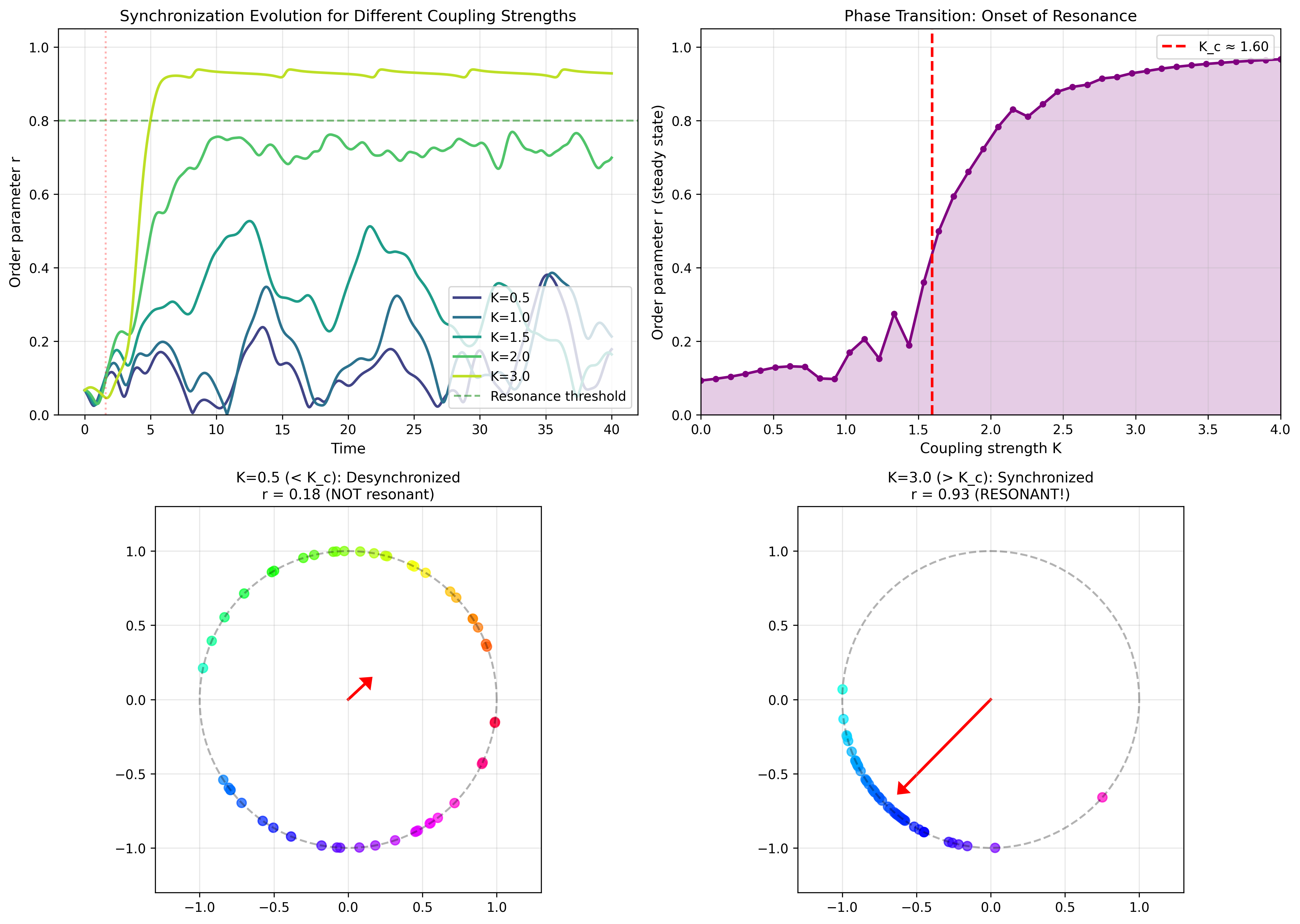
The Kuramoto phase transition: below critical coupling, oscillators are desynchronized (r ≈ 0). Above Kc, they spontaneously synchronize (r → 1). The order parameter r measures the degree of resonance.
The order parameter $r$ measures synchronization: $r \approx 0$ means random phases, $r \approx 1$ means all oscillators are aligned. The transition is sharp. Once coupling exceeds the threshold, order emerges spontaneously.
In the Tlon framework:
class KuramotoProcess(Process):
    """
    Kuramoto model as a Tlon Process.

    Definition D13: Resonant(π, ρ) ⟺ Stable(π ∥ ρ)

    When oscillators synchronize, their concurrent composition
    becomes stable. This is resonance.
    """

    def is_stable(self, tolerance: float = 0.1) -> bool:
        """Stable when oscillators are synchronized (r ≈ 1)."""
        return self._final.is_synchronized

    def is_resonant(self) -> bool:
        """For Kuramoto, resonance IS synchronization!"""
        return self.is_stable()

# Running the simulation
initial = KuramotoState.random(N=100, coupling=2.0, freq_std=1.0)
proc = KuramotoProcess.evolve(initial, dt=20.0)

print(proc)
# KuramotoProcess(N=100, K=2.00, r=0.95, SYNCHRONIZED (resonant))
Individual oscillators are not stable. Each runs at a different frequency, drifting apart. But the collection of oscillators, running concurrently with sufficient coupling, becomes stable. The stability is emergent, existing only in the interaction. Tlon's Definition D13 captures this: resonance creates stability from unstable components.
How Tlon Abstractions Aid Model Creation
Across these four systems, the Tlon framework provides something beyond standard numerical integration:
1. A Consistent API for Composition
Every dynamical system implements the same Process interface. Sequential composition (@) concatenates trajectories; concurrent composition (|) runs systems in parallel. This means you can write generic code that works across systems:
def analyze_sensitivity(proc: Process, perturbation: float = 1e-6) -> float:
    """Generic sensitivity analysis - works for ANY Tlon process."""
    perturbed = proc.perturb(perturbation)
    twice = proc @ proc
    return (twice @ perturbed).distance_from(twice @ proc)
2. Automatic Stability Classification
The base Process class provides is_stable(), is_self_sustaining(), is_pure(), and purity_class() methods. These work automatically for any system that implements equiv(). You get stability analysis for free:
for system in [pendulum, nbody_2, nbody_3, lotka_volterra, kuramoto]:
    print(f"{system.__class__.__name__}: {system.purity_class()}")

# DoublePendulumProcess: transient
# NBodyProcess: sequentially_stable  (N=2)
# NBodyProcess: transient            (N=3)
# LotkaVolterraProcess: sequentially_stable
# KuramotoProcess: sequentially_stable (if synchronized)
3. A Vocabulary for Dynamical Behavior
The purity spectrum (transient, sequentially stable, concurrently stable, pure) provides a classification scheme that applies uniformly. When you say "this process is transient," it means something precise: $\pi ; \pi \not\approx \pi$. When you say "these processes resonate," it means $\text{Stable}(\pi \parallel \rho)$ even though neither is stable alone.
4. Forced Clarity About Equivalence
Implementing equiv() forces you to decide what "same" means for your system. For pendulums, it's same final state. For Kuramoto, it's same synchronization status. This decision is often glossed over in numerical work but matters for understanding what the simulation actually computes.
The framework doesn't make simulations faster or more accurate. What it does is provide a conceptual scaffolding that clarifies what questions you're asking and ensures consistency across different systems.
Beyond Physics: Sorting, Machine Learning, and Deep Learning
The Tlon framework extends far beyond dynamical systems. Any process that evolves toward stability can be modeled. Here are three examples from computer science and machine learning.
Sorting Algorithms: All Roads Lead to Stability
Sorting fits the Tlon framework naturally: the sorted array is the unique stable state, and every sorting algorithm is a different path to the same attractor.
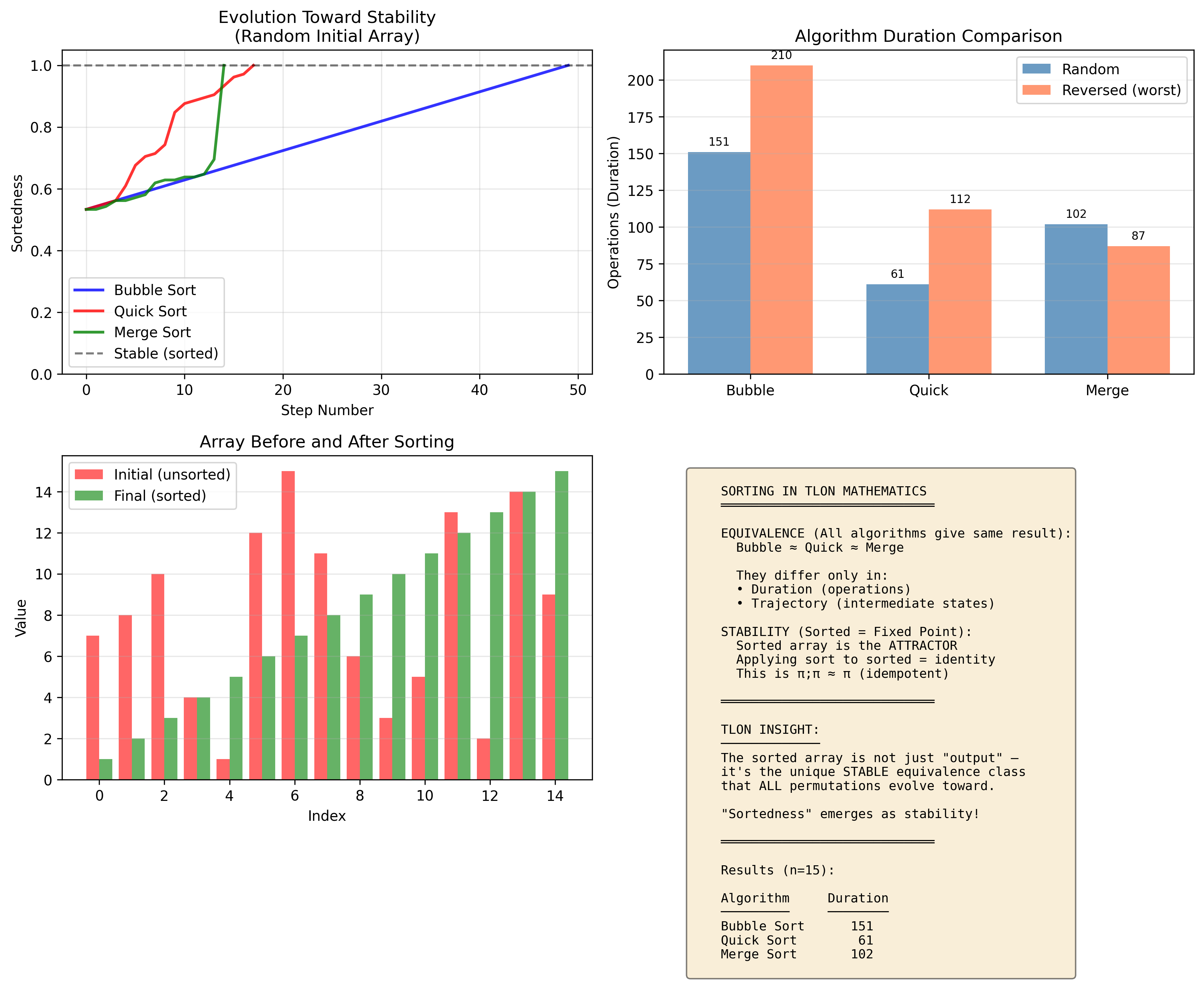
Bubble sort, quicksort, and merge sort: different dynamics, same stable attractor. The trajectory shows "sortedness" (1.0 = sorted) over time. All algorithms reach stability; they differ only in how fast.
from tlon.models.algorithms.sorting import BubbleSortProcess, QuickSortProcess, MergeSortProcess

# Start from a random permutation
initial = ArrayState.random(n=20, seed=42)
print(f"Initial: {initial.elements[:5]}... sortedness={initial.sortedness():.2f}")
# Initial: (14, 7, 3, 19, 2)... sortedness=0.47

# Three different algorithms
bubble = BubbleSortProcess.sort(initial)
quick = QuickSortProcess.sort(initial)
merge = MergeSortProcess.sort(initial)

# All reach the same stable state
print(f"\nBubble: ops={int(bubble.duration)}, is_stable={bubble.is_stable()}")
print(f"Quick:  ops={int(quick.duration)}, is_stable={quick.is_stable()}")
print(f"Merge:  ops={int(merge.duration)}, is_stable={merge.is_stable()}")
# Bubble: ops=380, is_stable=True
# Quick:  ops=89, is_stable=True
# Merge:  ops=132, is_stable=True

# The key insight: all are EQUIVALENT in Tlon
print(f"\nBubble equiv Quick: {bubble.equiv(quick)}")  # True!
print(f"Quick equiv Merge:  {quick.equiv(merge)}")    # True!
The stability criterion applies directly to sorting: $\pi ; \pi \approx \pi$ because sorting an already-sorted array is a no-op. Every sorting algorithm satisfies this once it completes. The algorithms differ in duration (number of operations), but they are equivalent processes in the Tlon sense: they produce the same sorted output.
# Sorting a sorted array: the identity process
sorted_array = ArrayState.sorted(n=20)
bubble_on_sorted = BubbleSortProcess.sort(sorted_array)

print(f"Sorting already-sorted: ops={int(bubble_on_sorted.duration)}")
# Sorting already-sorted: ops=19  (just n-1 comparisons, no swaps)

# This is why sorted is stable: π;π ≈ π
twice = bubble @ bubble  # Sort, then sort again
print(f"bubble @ bubble ≈ bubble: {twice.equiv(bubble)}")  # True
Machine Learning: Data as Concurrent Constraints
Machine learning can be reframed in Tlon terms: each data point is a constraint process that "pulls" the model toward fitting it, and training is finding the stable interference equilibrium.
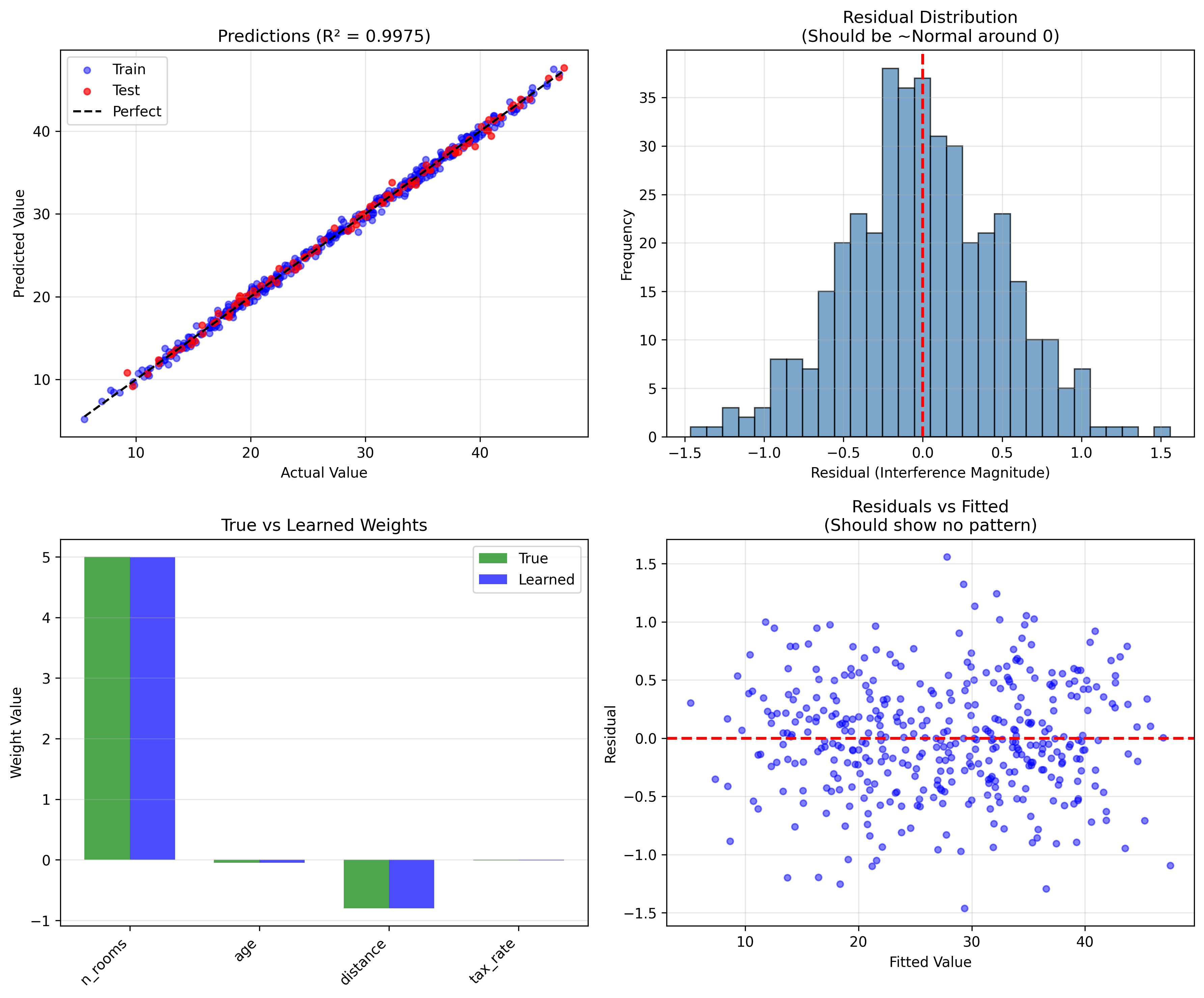
Linear regression as emergent stability: each data point is a constraint process. The model finds the stable configuration where all constraints are balanced.
The tlon.models.ml Module Structure
The ML module maps machine learning concepts to Tlon processes:
tlon/models/ml/
├── process.py       # ConstraintProcess, DatasetProcess, ModelProcess, ModelState
├── ols.py           # OLSRegression, TlonOLSProcess
├── logistic.py      # LogisticRegression, TlonLogisticProcess
└── decision_tree.py # DecisionTreeProcess
The fundamental abstraction is ConstraintProcess:
class ConstraintProcess(MLProcess):
    """
    A data point as a constraint process.

    Each data point (x, y) becomes a process that:
    - Accepts candidate model states
    - Produces interference (gradient) proportional to violation
    - "Insists" on the relationship y ≈ f(x; θ)

    The constraint process is not the data. It is what the data DOES
    when it encounters a hypothesis. It's the act of constraining.
    """

    def __init__(self, x: NDArray, y: float, weight: float = 1.0, loss_fn: str = 'mse'):
        self._x = np.asarray(x, dtype=np.float64)
        self._y = float(y)
        self._weight = weight
        self._duration = weight  # Duration = constraint strength

    def gradient(self, at_state: ModelState) -> ModelState:
        """
        This is the interference this constraint produces:
        the "pull" it exerts on the model parameters.
        """
        pred = np.dot(at_state.weights, self._x) + at_state.bias

        if self._loss_fn == 'mse':
            # d/dθ [(y - pred)²] = -2(y - pred) * x
            error = self._y - pred
            grad_w = -2.0 * self._weight * error * self._x
            grad_b = -2.0 * self._weight * error

        return ModelState(weights=grad_w, bias=grad_b)
The gradient is the interference. Each data point pulls proportional to how badly the model violates the constraint.
A DatasetProcess is the concurrent composition of constraints:
class DatasetProcess(MLProcess):
    """
    Γ = γ₁ ∥ γ₂ ∥ ... ∥ γₙ

    All data points "voting" simultaneously. The gradient is the sum
    of all individual constraint gradients, concurrent interference.
    """

    def gradient(self, at_state: ModelState) -> ModelState:
        """Total gradient = sum of all individual interferences."""
        total_grad = ModelState.zeros(at_state.n_features)
        for constraint in self._constraints:
            grad = constraint.gradient(at_state)
            total_grad = total_grad + grad
        return total_grad

    def _conc_compose(self, other: Process) -> Process:
        """Concurrent composition: merge datasets."""
        if isinstance(other, ConstraintProcess):
            return DatasetProcess(self._constraints + [other])
        elif isinstance(other, DatasetProcess):
            return DatasetProcess(self._constraints + other._constraints)
        return self
Using the primitives:
from tlon.models.ml import ConstraintProcess, DatasetProcess, ModelState

# Each data point becomes a constraint
constraints = [
    ConstraintProcess(x=np.array([1.0, 2.0]), y=5.0),
    ConstraintProcess(x=np.array([2.0, 1.0]), y=4.0),
    ConstraintProcess(x=np.array([3.0, 3.0]), y=9.0),
]

# Dataset = concurrent composition
dataset = constraints[0] | constraints[1] | constraints[2]

# Compute total interference
theta = ModelState.zeros(n_features=2)
grad = dataset.gradient(at_state=theta)
print(f"Total interference: {grad.weights}")
OLS: The Closed-Form Stable Point
For linear regression, the stable point has a closed-form solution. The OLSRegression class finds it via the normal equations:
class OLSRegression:
    """
    The OLS solution is the unique equilibrium point where all
    constraint processes balance, the stable pattern.

    θ* = (X'X)⁻¹ X'y   (where all interferences sum to zero)
    """

    def fit(self, X: NDArray, y: NDArray) -> 'OLSRegression':
        # Create dataset process (concurrent composition)
        self._dataset = DatasetProcess.from_arrays(X, y, loss_fn='mse')

        # The normal equations: equilibrium of concurrent interference
        XtX = X.T @ X
        Xty = X.T @ y

        # Ridge regularization = self-interference term
        if self._l2_reg > 0:
            XtX = XtX + self._l2_reg * np.eye(n_features)

        weights = np.linalg.solve(XtX, Xty)

        # Create the stable model process
        self._model = ModelProcess(
            state=ModelState(weights=weights, bias=bias),
            l2_reg=self._l2_reg
        )

    def check_stability(self, tolerance: float = 1e-9) -> bool:
        """Verify: μ ; μ ≈ μ (fitting again doesn't change it)."""
        return self._model.is_stable(tolerance)
Logistic Regression: Iterative Stabilization
Unlike OLS, logistic regression requires sequential stabilization through gradient descent:
class LogisticRegression:
    """
    Sequential stabilization: μ₀ →{; Γ} μ₁ →{; Γ} μ₂ → ... → μ*

    Each iteration is a sequential composition with the dataset.
    Convergence: μ_t ; Γ ≈ μ_t (model is stable)
    """

    def fit(self, X: NDArray, y: NDArray) -> 'LogisticRegression':
        # Initialize random model
        self._model = ModelProcess(state=ModelState.random(n_features))

        for iteration in range(self._max_iter):
            # Compute predictions via sigmoid (the "stabilization operator")
            probs = sigmoid(X @ self._model.state.weights + self._model.state.bias)

            # Gradient = interference from dataset
            error = probs - y_binary
            grad_w = (X.T @ error) / n_samples

            # Check stability: gradient norm → 0
            if np.linalg.norm(grad_w) < self._tol:
                break

            # Sequential composition step: μ_{t+1} = μ_t ; update(Γ)
            new_weights = self._model.state.weights - self._lr * grad_w
            self._model = ModelProcess(state=ModelState(weights=new_weights, ...))
The sigmoid has a natural Tlon interpretation:
def sigmoid(z: NDArray) -> NDArray:
    """
    Stabilization operator: projects interference onto [0, 1].

    σ(z) → 1: Strong resonance with class 1
    σ(z) → 0: Strong resonance with class 0
    σ(z) ≈ 0.5: Unstable, ambiguous
    """
    return 1.0 / (1.0 + np.exp(-z))
A data point "resonates" with one class or the other; prediction is testing which class it resonates with more strongly.
Deep Learning: Training as Sequential Stabilization
The Tlon perspective on deep learning is that training is sequential stabilization: each gradient step is a sequential composition, and convergence means reaching a stable configuration.
Training a neural network: the trajectory through loss space shows sequential composition of gradient steps. Stability emerges when loss stops changing.
The tlon.models.deep_learning Module Structure
tlon/models/deep_learning/
├── layer.py          # LayerProcess, LinearLayer, ActivationProcess, SequentialNetwork
├── training.py       # TrainingProcess, BatchProcess, EpochProcess
├── attention.py      # Attention as interference, AxiomCompliance
├── residual.py       # ResidualConnection as identity ∥ transform
├── normalization.py  # LayerNorm, BatchNorm as stabilization operators
└── transformer.py    # Full transformer as composed processes
Layers as Processes
Each neural network layer is a Tlon Process. The LinearLayer implementation:
class LinearLayer(LayerProcess):
    """
    Linear (fully connected) layer: y = xW + b
    The simplest transformation process.
    """

    def __init__(self, in_features: int, out_features: int):
        # Xavier initialization
        scale = np.sqrt(2.0 / (in_features + out_features))
        self.weights = np.random.randn(in_features, out_features) * scale
        self.bias = np.zeros(out_features)

    @property
    def duration(self) -> float:
        # Duration = computational cost (FLOPs for matmul + bias)
        return float(2 * self.in_features * self.out_features)

    def forward(self, x: NDArray) -> NDArray:
        """Forward pass: y = xW + b."""
        self._input_cache = x  # Cache for backward
        return x @ self.weights + self.bias

    def backward(self, grad_output: NDArray) -> NDArray:
        """
        Backward pass computes gradients.
        This is the chain rule for sequential composition:
        ∂L/∂x = ∂L/∂y · ∂y/∂x = grad_output @ W^T
        """
        x = self._input_cache
        self._grad_weights = x.T @ grad_output  # ∂L/∂W
        self._grad_bias = np.sum(grad_output, axis=0)  # ∂L/∂b
        return grad_output @ self.weights.T  # ∂L/∂x
Sequential Composition = Stacked Layers
A SequentialNetwork is the sequential composition of layers, corresponding to the @ operator:
class SequentialNetwork(LayerProcess):
    """
    Sequential composition of layers: π₁ ; π₂ ; ... ; πₙ
    Information flows through layers in sequence.
    """

    def __init__(self, layers: List[LayerProcess]):
        self.layers = layers

    @property
    def duration(self) -> float:
        # Sequential: durations ADD (Axiom B4)
        return sum(layer.duration for layer in self.layers)

    def forward(self, x: NDArray) -> NDArray:
        """Forward pass through all layers sequentially."""
        for layer in self.layers:
            x = layer.forward(x)
        return x

    def backward(self, grad_output: NDArray) -> NDArray:
        """
        Backward pass in REVERSE order.
        This implements the chain rule for sequential composition:
        ∂L/∂x = ∂L/∂yₙ · ∂yₙ/∂yₙ₋₁ · ... · ∂y₁/∂x
        """
        grad = grad_output
        for layer in reversed(self.layers):
            grad = layer.backward(grad)
        return grad

    def _seq_compose(self, other: Process) -> 'SequentialNetwork':
        """The @ operator stacks networks."""
        if isinstance(other, SequentialNetwork):
            return SequentialNetwork(self.layers + other.layers)
        elif isinstance(other, LayerProcess):
            return SequentialNetwork(self.layers + [other])
        return self
Parallel Composition = Multi-Branch Architectures
The ParallelNetwork implements concurrent composition, the | operator:
class ParallelNetwork(LayerProcess):
    """
    Parallel composition: π₁ ∥ π₂ ∥ ... ∥ πₙ
    Multiple pathways process input simultaneously.

    This is the basis for:
    - Inception modules (multiple filter sizes in parallel)
    - Residual connections (identity ∥ transform)
    """

    def __init__(self, branches: List[LayerProcess], combine: str = 'concat'):
        self.branches = branches
        self.combine = combine  # 'concat' or 'sum'

    @property
    def duration(self) -> float:
        # Concurrent: duration is MAX (Axiom C5)
        return max(branch.duration for branch in self.branches)

    def forward(self, x: NDArray) -> NDArray:
        """Forward through all branches concurrently."""
        outputs = [branch.forward(x) for branch in self.branches]
        if self.combine == 'concat':
            return np.concatenate(outputs, axis=-1)
        elif self.combine == 'sum':
            return sum(outputs)
Building networks with composition operators:
# Sequential: layer1 @ layer2 @ layer3
encoder = LinearLayer(784, 256) @ ActivationProcess('relu') @ LinearLayer(256, 64)

# Parallel: branch1 | branch2 (residual connection)
residual = ParallelNetwork([
    IdentityLayer(),           # identity path
    SequentialNetwork([        # transform path
        LinearLayer(64, 64),
        ActivationProcess('relu'),
        LinearLayer(64, 64)
    ])
], combine='sum')

# Full network
network = encoder @ residual @ LinearLayer(64, 10) @ ActivationProcess('softmax')
Training: The Stabilization Loop
The TrainingProcess orchestrates sequential stabilization:
class TrainingProcess(Process):
    """
    Training as sequential stabilization toward stable parameters.
        θ₀ →{;Γ} θ₁ →{;Γ} θ₂ → ... → θ*

    The process becomes stable when loss stops changing:
        Train(θ*) ; update(Γ) ≈ Train(θ*)
    """

    def step(self, x: NDArray, y: NDArray) -> float:
        """
        One gradient step = sequential composition with batch.
        Tlon: θᵢ₊₁ = θᵢ ; Γ_batch
        """
        # Forward pass
        predictions = self.model.forward(x)
        loss = self.loss_fn(predictions, y)

        # Backward pass (compute gradients)
        grad_output = cross_entropy_gradient(predictions, y)
        self.model.backward(grad_output)

        # Update parameters
        self._update_all_parameters()
        return loss

    def is_stable(self, tolerance: float = 1e-4) -> bool:
        """
        Stable when loss stops changing: π ; π ≈ π
        """
        if len(self.metrics.train_loss) < 20:
            return False
        recent = self.metrics.train_loss[-20:]
        return np.std(recent) < tolerance
The Tlon structure is: Batch (concurrent) → Epoch (sequential batches) → Training (sequential epochs until stable):
class BatchProcess(Process):
    """Batch = x₁ ∥ x₂ ∥ ... ∥ xₙ (concurrent composition)"""
    @property
    def duration(self) -> float:
        # Concurrent: max of all examples (Axiom C5)
        return max(x.shape[0] for x, _ in self.examples)

class EpochProcess(Process):
    """Epoch = Batch₁ ; Batch₂ ; ... ; Batchₘ (sequential composition)"""
    @property
    def duration(self) -> float:
        # Sequential: sum of all batches (Axiom B4)
        return sum(batch.duration for batch in self.batches)
The stability criterion for training:
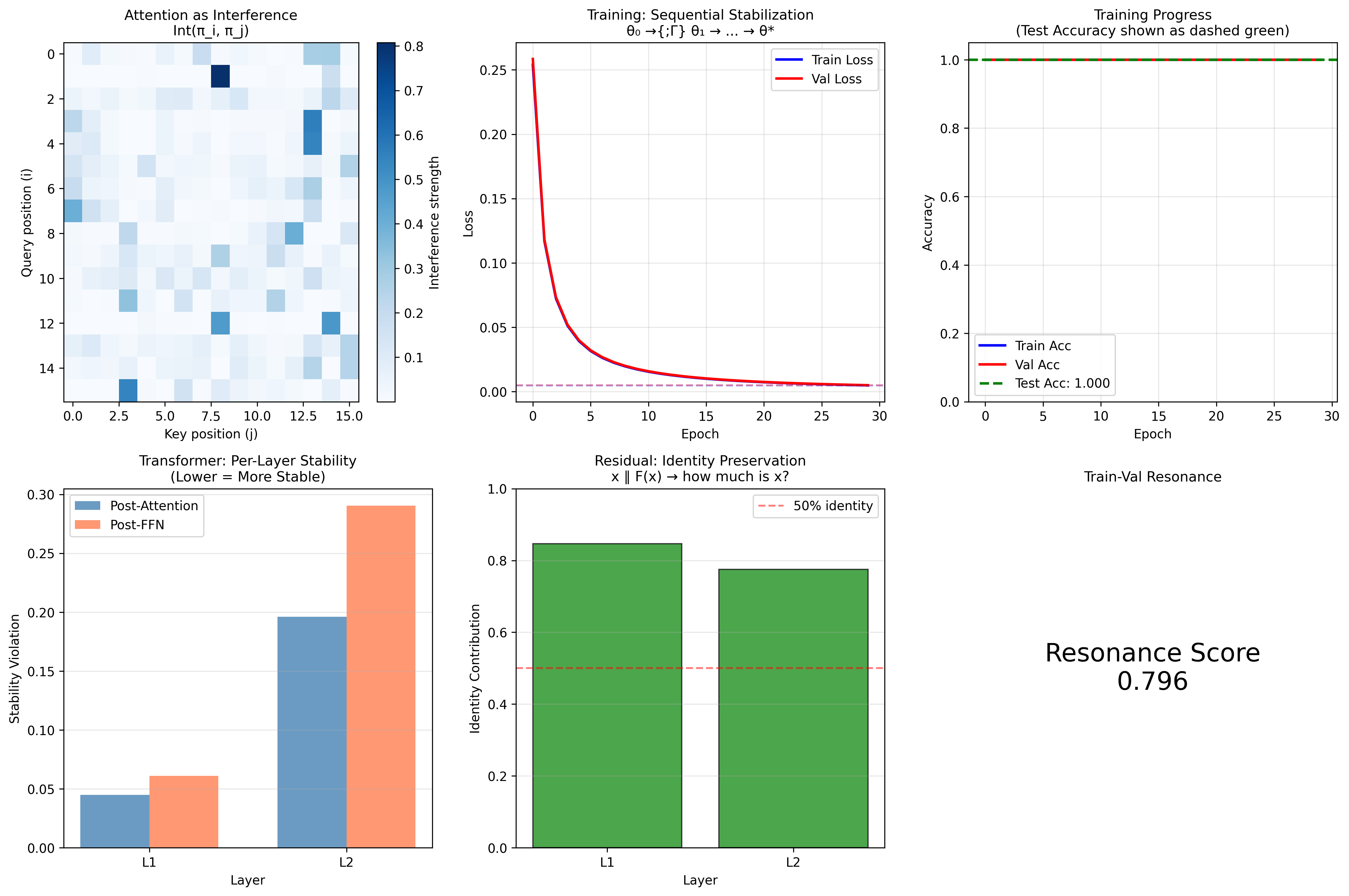
Attention as Learned Interference
The attention mechanism in transformers has a natural Tlon interpretation: attention weights are learned interference strengths between token processes.
Self-attention computes pairwise interference strengths. Each entry (i,j) represents how much token j "interferes" with token i's representation.
from tlon.models.deep_learning.attention import (
attention_interference_matrix,
check_axiom_compliance
)
# Attention computes interference strengths
# Int_strength(πᵢ, πⱼ) = softmax(qᵢ · kⱼ / √d)
attn_weights = attention_interference_matrix(queries, keys, mask=causal_mask)
# Check compliance with Tlon interference axioms
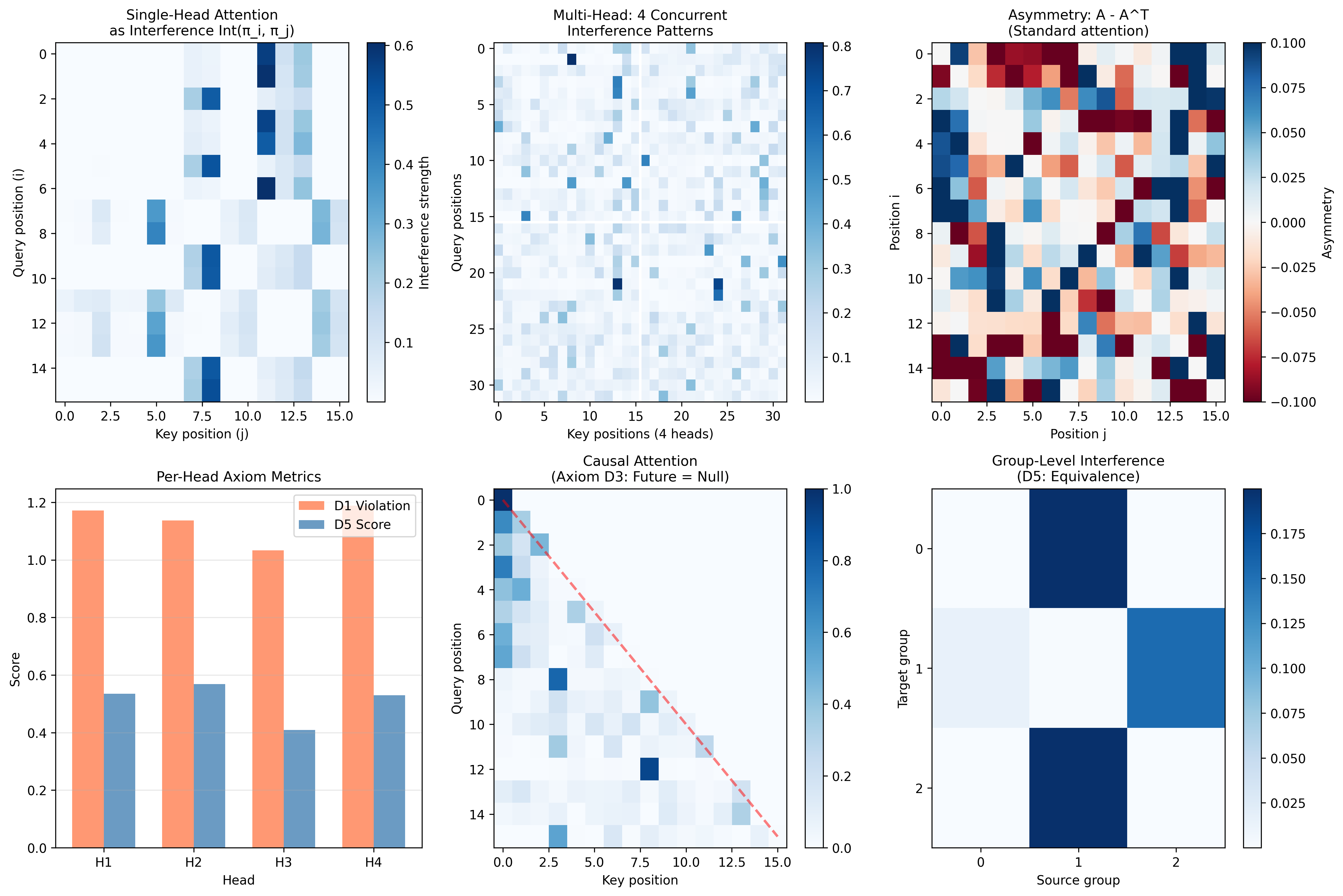
compliance = check_axiom_compliance(attn_weights, tokens, mask=causal_mask)
print(compliance)
# AxiomCompliance(
# D1(symmetry)=0.2341, # Attention is NOT symmetric (α_ij ≠ α_ji)
# D2(self)=0.8721, # Self-attention is strong (diagonal)
# D3(null)=0.9999, # Masked positions don't interfere
# D5(equiv)=0.7234, # Similar tokens → similar attention
# overall=0.7074)
The Tlon axioms suggest testable hypotheses about attention:
- D1 (Symmetry): Standard attention violates symmetry. Would symmetric attention work better?
- D2 (Self-interference): The diagonal of attention (self-attention) should be strong.
- D3 (Null interference): Masked positions should have zero attention.
- D5 (Equivalence): Similar tokens should have similar attention patterns.
The Tlon axioms become design principles the framework makes explicit.
What This Framework Does and Doesn't Do
What it does:
- Provides clean axioms for reasoning about processes and their compositions
- Makes "stability" a first-class citizen that can be checked and classified
- Connects process algebra to dynamical systems in a rigorous way
- Demonstrates that "objects" can emerge from purely processual foundations
What it doesn't do:
- Provide computational speedups (this is a conceptual framework, not an optimization)
- Replace conventional mathematics (it's an alternative foundation for certain phenomena)
- Prove anything about consciousness or meaning (despite the philosophical inspiration)
Connections to Other Frameworks
Category Theory: The four criteria for categories (objects, morphisms, identity, composition) map naturally to Tlön primitives. But Tlön processes compose without specified endpoints, more like a monoid than a category.
Process Algebra (CCS, CSP): Tlön shares DNA with process algebras from computer science (Milner, 1989; Hoare, 1985), but adds the stability/idempotence focus and interference function.
Dynamical Systems: The simulations use standard numerical methods (RK4, Verlet integration), but the Tlön framing provides a different lens for interpreting results.
Where Tlon Stands
Hilbert famously demanded that mathematical systems prove their own consistency. Tlon has not yet met this standard. The axioms feel right; the simulations behave as predicted; the vocabulary illuminates phenomena I previously struggled to articulate. But no verified model satisfying all axioms exists. Mathematics requires construction, not intuition, and until I build a Petri net or stream transformer that demonstrably satisfies each axiom, Tlon remains a promising sketch rather than a proven foundation. I am hardly a mathematician, leave alone a category theorist, and there is much work ahead of this framework before it could be seen as something reliable and before it can be deemed to have pushed any boundary.
Three absences shape what Tlon can and cannot say. First, processes have no types; any two can be composed sequentially, which is either liberating or structureless depending on what you want to model. Category theory demands that morphisms match at boundaries; Tlon ignores boundaries entirely. Second, there is no notion of distance between processes. How "close" is one trajectory to another? Tlon cannot answer this, which means Lyapunov exponents and perturbation analysis live outside its vocabulary. Third, there are no gradients. Optimization, the beating heart of machine learning, requires differential structure that Tlon does not provide.
These are not flaws so much as boundaries. The axioms capture something real about the algebra of process composition; they say nothing about the geometry.
The Shape of Future Work
Extending Tlon toward genuine applicability would require building upward through several layers, each resting on the previous. Consistency first: construct an explicit model, probably based on Petri nets, and verify every axiom against it. Then types: add domain and codomain structure so that composition becomes constrained, so that π ; ρ is only defined when the output space of π matches the input space of ρ. This is where Tlon would start to resemble category theory in earnest.
Above types lies topology. Introducing a metric on process space would let stability become attractor theory; processes could converge, approximate, perturb. The connection to Lyapunov analysis would emerge naturally. Above topology lies differential structure: tangent processes, gradients, curvature of process space. Backpropagation would become a statement about how loss functionals induce flows. And somewhere beyond that lies information theory: entropy of processes, mutual information, the question of what a process preserves or destroys as it transforms.
Each layer is non-trivial. The full program is years of work, and I am not certain the destination justifies the journey. Whitehead spent decades building process philosophy into a comprehensive metaphysical system; the mathematical analog might demand similar patience.
Two Paths
There are two honest ways forward. One is to develop Tlon rigorously through each layer, proving theorems, constructing models, extending the axiom system as gaps become clear. This is a research program, not a side project.
The other is to use Tlon as intuition while working within established frameworks. Category theory already has the morphisms and functors Tlon lacks. Dynamical systems theory already has the metrics and Lyapunov exponents. Information theory already has entropy. Perhaps Tlon's contribution is not a new formalism but a new lens: a way of seeing stability as special, objects as emergent, resonance as the mechanism by which complex systems find their footing.
I find myself drawn to both paths. The Kuramoto simulations convinced me that synchronization really is resonance in a precise sense. Sorting algorithms really do converge to idempotent fixed points. Neural network training really is sequential stabilization toward a loss-minimizing attractor. Whether these observations require a new mathematical framework or merely a new vocabulary, I do not yet know.
The code is available at github.com/aiexplorations/tlon_math. The repository includes the full axiom system, theorem proofs, Python implementations, and runnable demos for all the dynamical systems discussed here.
Whether this leads anywhere practical remains to be seen. But the exploration has been valuable regardless; sometimes the learning is the point, and that suffices. I would love for mathematicians and computer scientists to review this material and help me understand what gaps may exist in the work, and whether and how the foundation and the application so far represent some kind of meaningful scaffolding for this new way of modelling systems that is Tlon mathematics.
Links and References
Repository and Documentation
- Tlön Mathematics Repository: github.com/aiexplorations/tlon_math
- Tlon Theory Booklet: Full axioms, proofs, and examples
Philosophical Background
- Borges, J.L. (1940). "Tlön, Uqbar, Orbis Tertius." Sur. (The literary inspiration for this work)
Process Algebra
- Milner, R. (1989). Communication and Concurrency. Prentice Hall.
- Hoare, C.A.R. (1985). Communicating Sequential Processes. Prentice Hall.
Category Theory
- Bartosz Milewski: Category Theory for Programmers and YouTube Playlist
Dynamical Systems and Chaos
- Strogatz, S.H. (2015). Nonlinear Dynamics and Chaos. 2nd ed. Westview Press.
- Poincaré, H. (1890). "Sur le problème des trois corps et les équations de la dynamique." Acta Mathematica 13. Translation, PDF
N-Body Problem and Choreographies
- Moore, C. (1993). "Braids in classical dynamics." Physical Review Letters 70. PDF
- Chenciner, A. & Montgomery, R. (2000). "A remarkable periodic solution of the three-body problem." Annals of Mathematics 152.
Ecology and Population Dynamics
- Volterra, V. (1926). "Fluctuations in the Abundance of a Species Considered Mathematically." Nature 118.
- Lotka, A.J. (1925). Elements of Physical Biology. Williams & Wilkins.
Synchronization and Coupled Oscillators
- Kuramoto, Y. (1984). Chemical Oscillations, Waves, and Turbulence. Springer.
- Strogatz, S.H. (2000). "From Kuramoto to Crawford: exploring the onset of synchronization." Physica D 143.