A clock is a computer that performs modular arithmetic. When the hour hand points to 11 and three hours pass, it points to 2, not 14. The clock face encodes the fact that hours wrap around; there is no hour 14, only hour 2. This wrapping is modulo 12: $11 + 3 = 14 \equiv 2 \pmod{12}$.
A clock face is circular because the arithmetic is circular. Position on the circle encodes the hour; adding time means rotating around the circle. This Welch Labs video on grokking uses this example to explain something surprising that researchers discovered when they trained a neural network on modular addition.
The model OpenAI's team built as per the Grokking paper was tiny, a small transformer learning to compute $(a + b) \mod p$ for some prime $p$. It memorized the training examples quickly and the model loss dropped quite fast, but generalization was poor despite the loss being low. It turns out that someone on the OpenAI team left the model to continue training and came back to the unexpected discovery that performance on held-out test sets was excellent. Long after the training was deemed to be complete, the model had actually "learned" or "grokked".
When they visualized the learned representations, the OpenAI team found interesting weight representations in the layers of the model. The numbers 0 through $p-1$ were arranged around circular patterns in the weight space, with Fourier components encoding position on the circle. The model had independently discovered that addition mod $p$ lives on a circle, just like we discussed in the clock example at the start of this blog. The team had found Lissajous figures in the weight visualizations - the kind you will see on an oscilloscope in a signals laboratory. These were trigonometric embeddings, the same mathematical structure behind positional encodings in transformers, but discovered autonomously for this specific task.
I watched this video months with rapt attention a few days ago, months after I had started building what would become ToDACoMM. Here was evidence that models learn structured geometric representations, and I had been building tools to measure exactly that kind of structure.
My own intuitions came from a few failed experiments on topological data analysis (TDA). I had figured that if only some vectors were represented significantly in vector space there would be voids in the data that was being fed to LLMs, and if the different attention layers and heads we described within models were learning from this data, they too would be developing such voids and other patterns with interesting and non trivial topologies in their weights. It followed that I should explore the nature of the geometry and topology of the weights, because this is where some insight into how models may learn, was likely to be present. I am sure I am not the first guy to think of this, and in fact there has been a lot of research in topological deep learning and TDA for deep learning models. TDA is itself a very old consideration, decades old if not centuries, but it seemed very topical and relevant.
Two Ways of Seeing
In fact, there are two lenses through which I have come to see neural networks, and they are older than neural networks themselves.
The first is dynamical systems. Training is gradient flow on the loss landscape $\mathcal{L}(\theta)$, a trajectory through parameter space following $\dot{\theta} = -\nabla_\theta \mathcal{L}$. Deep learning practitioners know this intuitively: the optimizer moves through weight space, gets stuck in local minima, escapes via momentum or learning rate schedules, eventually settles somewhere useful. Grokking is a phase transition where the system escapes a memorization basin and finds a generalizing solution.
The forward pass is also dynamical. Layer by layer, representations evolve through a composition of nonlinear maps $f_L \circ f_{L-1} \circ \cdots \circ f_1$. Each layer transforms the geometry of the activation space. In deep learning terms: early layers extract low-level features, later layers compose them into higher-level representations. In dynamical systems terms: the input evolves through a sequence of nonlinear transformations, each reshaping the space.
The second is topology. Where dynamical systems ask "how does this evolve?", topology asks "what is the shape of the space it evolves in?"
For deep learning practitioners, think of it this way: when you visualize embeddings with t-SNE or UMAP, you see clusters (similar items grouped together) and sometimes you see loops or manifold structure. Topology formalizes this. Persistent homology captures shape at multiple scales: it tracks how connected components ($H_0$, roughly "clusters"), loops ($H_1$, roughly "circular patterns"), and voids ($H_2$) appear and disappear as you vary a distance threshold. The persistence of a feature measures its significance; noise creates short-lived features, real structure persists.
These two perspectives are not separate. The shape of a space constrains what can happen within it. If representations cluster tightly, certain distinctions become hard to learn. If they spread into loops or manifolds, certain patterns become natural to encode. Measuring the topology of learned representations tells us something about what the training dynamics carved out.
Reading Shape from Points
Imagine scattering a handful of coins on a table. Some land close together, others far apart. If you squint, you might see clusters; coins that fell near each other form natural groups. If you arranged them deliberately in a circle, you would see the ring shape even though the coins themselves are just points. This isn't dissimilar to finding clusters as you might in some data, except we're not looking for decision boundaries in topology.
Persistent homology is a method for detecting such "structure" algorithmically. The idea is simple: grow a ball around each point, starting from radius zero. At first, each point is isolated, and there are as many separate components as there are points. As the radius increases, balls begin to overlap. When two balls touch, their points become connected and two components merge into one. These are connected components. Keep growing, and eventually everything connects into a single blob.
The trick is to watch what happens along the way. Components that merge quickly were close together; they were probably part of the same cluster. Components that persist as separate until late in the process were genuinely far apart. A feature that appears and disappears quickly is likely noise, and a feature that persists across a wide range of radii reflects real structure in the data. The latter mechanism is quite intuitive if you had begun to imagine these balls which we grew intersecting and becoming connected components in your mind's eye.
This presence of features across a wide range of radii is the "persistent" in persistent homology: we care not just about what features exist, but how long they last.
Loops work similarly. As balls grow and overlap, they sometimes form closed rings before filling in completely. If five points are arranged in a pentagon, the balls will first connect into a cycle, and only later will the interior fill in when the radius grows large enough. The cycle is born when the ring closes and dies when the interior fills. A cycle that persists for a long time indicates genuine circular structure; one that dies immediately was just an accident of the point configuration.
The Vietoris-Rips complex is the specific construction that makes this precise, rather than just an arbitraty mechanism. At each radius $\epsilon$, we connect points that are within distance $\epsilon$ of each other. As $\epsilon$ grows from zero to infinity, features appear and disappear. Ripser is an algorithm, implemented as a Python library, that computes this efficiently even for thousands of points in dozens of dimensions. It returns a list of birth-death pairs: each pair records when a topological feature was born (at what radius) and when it died. The difference, death minus birth, is the persistence.
In the language of homology: $H_0$ counts connected components (clusters), $H_1$ counts loops (circular patterns), and $H_2$ counts voids (hollow cavities). For analyzing neural network representations, $H_0$ and $H_1$ are the most informative, because we are dealing with layers in neural networks. High $H_0$ persistence means the points are spread out, with well-separated clusters. High $H_1$ persistence means there are genuine circular or periodic structures in the geometry.
When I run Ripser on the activations of a transformer layer, I am asking: what is the shape of the space these representations occupy? Are they clustered or diffuse? Do they trace out loops? The answers turn out to differ dramatically between encoder and decoder architectures.
What Models Learn
Neural network training is iterative error correction: forward pass, loss computation, backpropagation, weight update. The dynamics converge (when they converge) to regions of weight space where the model's internal representations support accurate prediction.
What are these representations? For a transformer processing text, each layer produces activations $h^{(l)} \in \mathbb{R}^{d}$ for each token. If you've worked with transformers, you know these aren't arbitrary vectors. The embedding layer maps tokens to a learned space where semantic similarity corresponds to geometric proximity; "king" and "queen" are closer than "king" and "banana". Attention layers then transform these representations based on context, and feedforward layers apply nonlinear transformations.
For the model to generalize, it must organize representations so that similar contexts cluster, syntactic patterns are geometrically encoded, and semantic relationships become spatial. The model learns a representation manifold, a high-dimensional space where the structure of language is reflected in geometry.
This manifold is shaped by the training dynamics. Each gradient update pushes and pulls the representation geometry, separating what should be distinguished, clustering what should be similar. When we measure the topology of trained representations, we are measuring what the optimization process carved out.
The Grokking paper showed one such carving, Fourier circles for modular arithmetic. Circles are the right geometry for cyclic groups. What shapes do language models carve? What is the topology of GPT-2's representation space versus BERT's? This is what ToDACoMM was built to investigate.
The Metrics: What We Measure and Why
Before diving into the tool and its findings, it helps to understand what we are actually measuring and what each metric tells us about neural network representations.
Topological Metrics
H0: Connected Components (Cluster Structure)
H0 counts how many separate "islands" exist in the data at different scales. If you imagine the point cloud of neural network activations, H0 asks: how many distinct clusters are there, and how far apart are they?
When H0 persistence is high, representations are spread out with well-separated groups. When it is low, everything clusters together. For a classifier, you might expect H0 to increase through the network as the model separates different classes into distinct regions. For a language model, the pattern is more complex; representations must both cluster (similar meanings together) and spread (different contexts distinguishable).
H1: Loops (Cyclic Structure)
H1 counts circular patterns in the data. If representations trace out a ring or cycle as you vary some property of the input, H1 detects it. The grokking model learned circles because modular arithmetic is inherently cyclic; H1 would capture this.
In language models, H1 might reflect periodic patterns: days of the week forming a cycle, verb conjugations with recurring structure, or the periodicity inherited from positional encodings. High H1 persistence means these cycles are robust features of the representation geometry, not artifacts.
Persistence: Separating Signal from Noise
Not all topological features are meaningful. Some clusters merge quickly; some loops fill in immediately. Persistence measures how long a feature survives as we vary the scale parameter. A feature with high persistence, one that appears early and dies late, reflects genuine structure. A feature with low persistence is likely noise.
When we report "total H0 persistence" or "max H1 lifetime," we are summarizing how much robust structure exists. A model with high total persistence has carved out a more structured representation space.
Geometric Metrics
Topology tells us about shape, but not about scale or density. The geometric metrics fill this gap.
Intrinsic Dimension
A 768-dimensional activation vector does not actually use all 768 dimensions. The data lies on a lower-dimensional manifold embedded in this high-dimensional space. Intrinsic dimension estimates the true dimensionality of this manifold.
If GPT-2's embeddings have intrinsic dimension 32, the model is using roughly 32 independent degrees of freedom to encode token meanings, despite the 768-dimensional container. Watching intrinsic dimension change through layers reveals how the network compresses or expands its representation complexity.
Hubness
In high-dimensional spaces, distance behaves strangely. Some points become "hubs," appearing in many other points' nearest-neighbor lists simply due to the geometry of high dimensions, not because they are semantically central. This is the curse of dimensionality manifesting in k-NN structure.
A hubness score of 1.0 indicates uniform k-NN structure: no pathological hubs. Scores above 1.0 indicate hub points exist. For neural network representations, we want hubness near 1.0; it means the learned space has healthy geometry where nearest-neighbor relationships are meaningful, not artifacts of dimensionality.
Distance Distribution
How far apart are representations? The mean, variance, and shape of the k-NN distance distribution tell us whether points are tightly packed, spread out, or somewhere in between. Tracking this through layers reveals whether the network expands representations (spreading them apart) or compresses them (pulling them together).
Why These Metrics Together
No single metric tells the full story. Intrinsic dimension might drop while H0 persistence rises; the network is compressing to fewer dimensions but spreading points within that subspace. Hubness might normalize while H1 count stays constant; the k-NN structure improves without changing the topological complexity.
The combination of topological metrics (H0, H1, persistence) and geometric metrics (intrinsic dimension, hubness, distance distribution) provides a multi-faceted view of representation geometry. Together, they characterize what gradient descent carved out.
Measuring the Carved Space
ToDACoMM (Topological Data Analysis Comparison of Multiple Models) characterizes transformer representations using persistent homology. The pipeline:
- Extract activations ${h_i^{(l)}}$ at each layer $l$ for $n$ text samples
- Project to $k=50$ principal components (retaining ~95% variance)
- Compute Vietoris-Rips persistent homology via Ripser
- Extract topological summaries: total persistence, max lifetimes, feature counts
System Architecture

Quick Start
# Install
git clone https://github.com/aiexplorations/todacomm
cd todacomm
pip install -e ".[dev]"

# Analyze a single model
todacomm run --model gpt2 --samples 500

# Compare encoder vs decoder
todacomm run --models gpt2,bert --samples 500

# Use all layers (14 for GPT-2)
todacomm run --model gpt2 --layers all

# GPU acceleration
todacomm run --model gpt2 --device cuda
Supported Models
ToDACoMM includes 20+ pre-configured transformer models under 1B parameters, plus configurable MLP architectures:
| Family | Models | Parameters | Type |
|---|---|---|---|
| GPT-2 | gpt2, gpt2-medium, distilgpt2 | 82-354M | Decoder |
| BERT | bert, distilbert | 66-110M | Encoder |
| Pythia | pythia-70m, pythia-160m, pythia-410m | 70-410M | Decoder |
| SmolLM2 | smollm2-135m, smollm2-360m | 135-360M | Decoder |
| Qwen | qwen2-0.5b, qwen2.5-0.5b, qwen2.5-coder-0.5b | 500M | Decoder |
| OPT | opt-125m, opt-350m | 125-350M | Decoder |
| MLP | shallow_2, shallow_3, medium_4, medium_5, deep_6 | <1M | Feedforward |
MLP models support MNIST, FashionMNIST, and UCI tabular datasets (iris, wine, digits, breast_cancer). Custom HuggingFace models: todacomm run --hf-model <model-name> --num-layers <N>
Output Structure
Each experiment generates:
experiments/<model>_tda_<timestamp>/
├── runs/run_0/
│   ├── tda_summaries.json      # H0/H1 metrics per layer
│   ├── metrics.json            # Perplexity, accuracy
│   ├── tda_interpretation.md   # Human-readable analysis
│   └── visualizations/
│       ├── tda_summary.png     # 6-panel metric overview
│       ├── layer_persistence.png
│       └── betti_curves.png
└── reports/
    └── experiment_report.md    # Full analysis report
The visualization plots show:
- tda_summary.png: H0/H1 count, total persistence, and max lifetime across layers
- layer_persistence.png: Side-by-side comparison of H0 vs H1 evolution
- betti_curves.png: Feature count trends through the transformer stack
TDA Methodology Details
The dimensionality reduction step is practical: persistent homology on 768-dimensional point clouds is computationally prohibitive. PCA to 50 dimensions preserves most of the variance while making computation tractable. This is a tradeoff; we might miss structure in the discarded components, but the patterns that emerge are robust across different choices of $k$.
The Vietoris-Rips complex works by growing balls around each point. At radius $\epsilon = 0$, each point is its own connected component. As $\epsilon$ grows, balls overlap, points connect, and the topology changes. The algorithm tracks when topological features (components, loops) are born and when they die. A feature that persists across a wide range of $\epsilon$ is likely real structure; a feature that dies quickly is likely noise.
The key metrics:
-
H0 Total Persistence: Sum of lifetimes of all connected components. In deep learning terms: how spread out are the representations? If activations form tight clusters, H0 is low. If they spread across the space, H0 is high.
-
H1 Total Persistence: Sum of lifetimes of all loops. In deep learning terms: are there circular or periodic patterns in the representation geometry? High H1 indicates the model has learned representations with loop structure.
-
Expansion Ratio: $\text{peak}(H_0) / H_0^{(0)}$, where $H_0^{(0)}$ is the embedding layer. This captures how much the geometry transforms through the network. A ratio of 1x means the representation geometry doesn't change much from embedding to final layer. A ratio of 100x means dramatic expansion.
I analyzed ten models across five architecture families (GPT-2, BERT, Pythia, SmolLM2, Qwen), each processing 500 WikiText-2 samples. Bootstrap resampling (B=100) provided 95% confidence intervals.
Beyond Transformers: MLPs as a Baseline
Before examining transformer topology in depth, it helps to understand what TDA reveals about simpler architectures. ToDACoMM now supports multi-layer perceptrons, the feedforward networks that predate attention mechanisms by decades. Without the recombinatory complexity of attention, the geometric transformations in MLPs are more direct, providing a cleaner baseline for interpretation.
A 3-layer MLP trained on MNIST (784 → 256 → 128 → 10) shows something quite different from transformers. The input layer, a 784-dimensional space of pixel intensities, has an intrinsic dimension around 15; the MNIST manifold is far smaller than the ambient space suggests. Through the hidden layers, this dimension compresses further, dropping to approximately 7 by the output layer. The network learns a progressively lower-dimensional representation as it approaches the 10-class decision boundary.
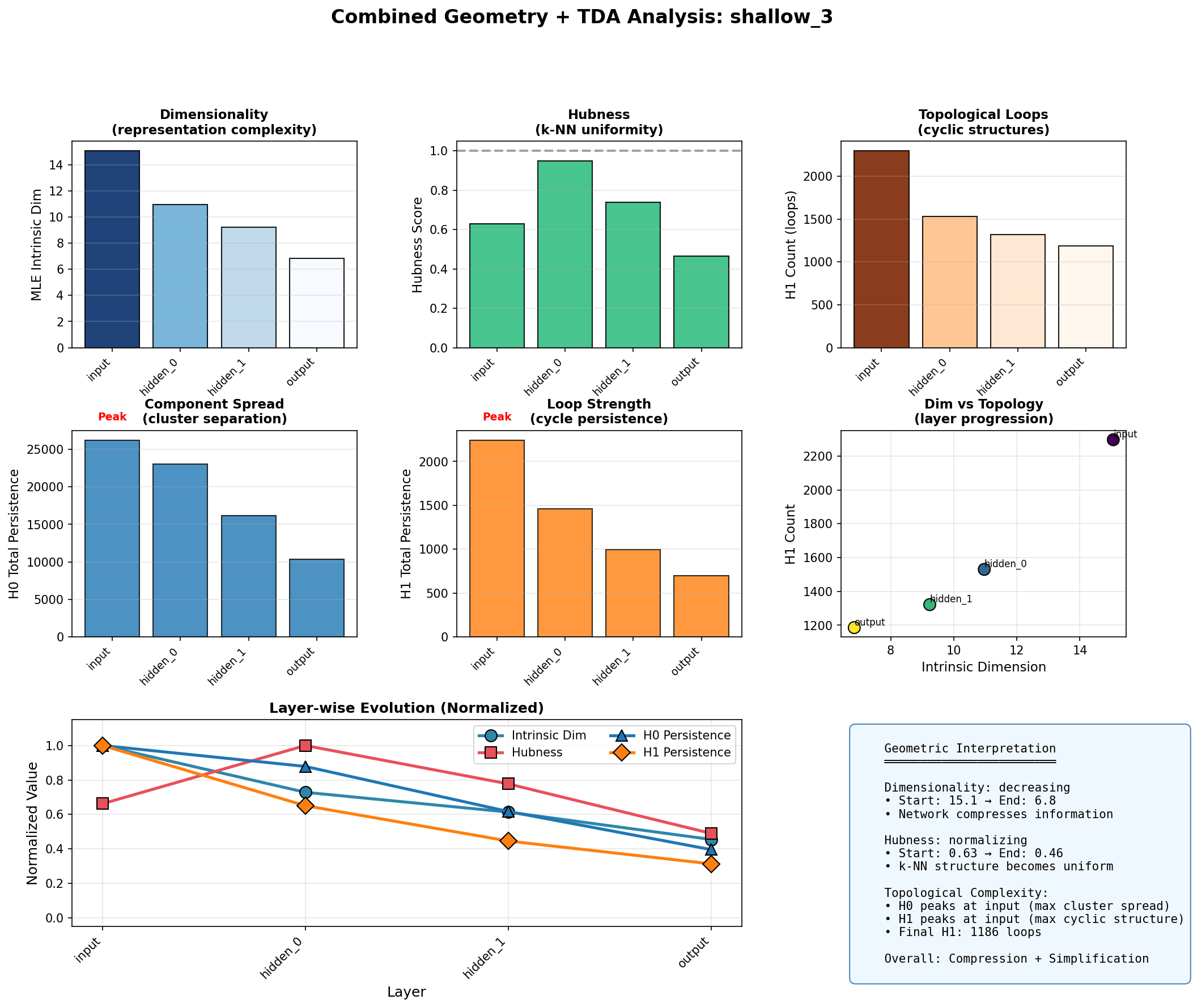
The hubness score tells a parallel story. In high-dimensional spaces, some points become "hubs", appearing disproportionately often in other points' nearest-neighbor lists due to the concentration of measure. Good representations should have hubness near 1.0, indicating uniform k-NN structure. The MLP achieves this; starting at 0.63 and remaining below 1.0 throughout, the network maintains uniform neighborhood structure as it compresses.
Both H0 and H1 persistence decrease monotonically through the MLP layers. The input has the highest topological complexity; the output has the lowest. This is compression in the topological sense: the network simplifies the representation space as it projects toward class centroids.
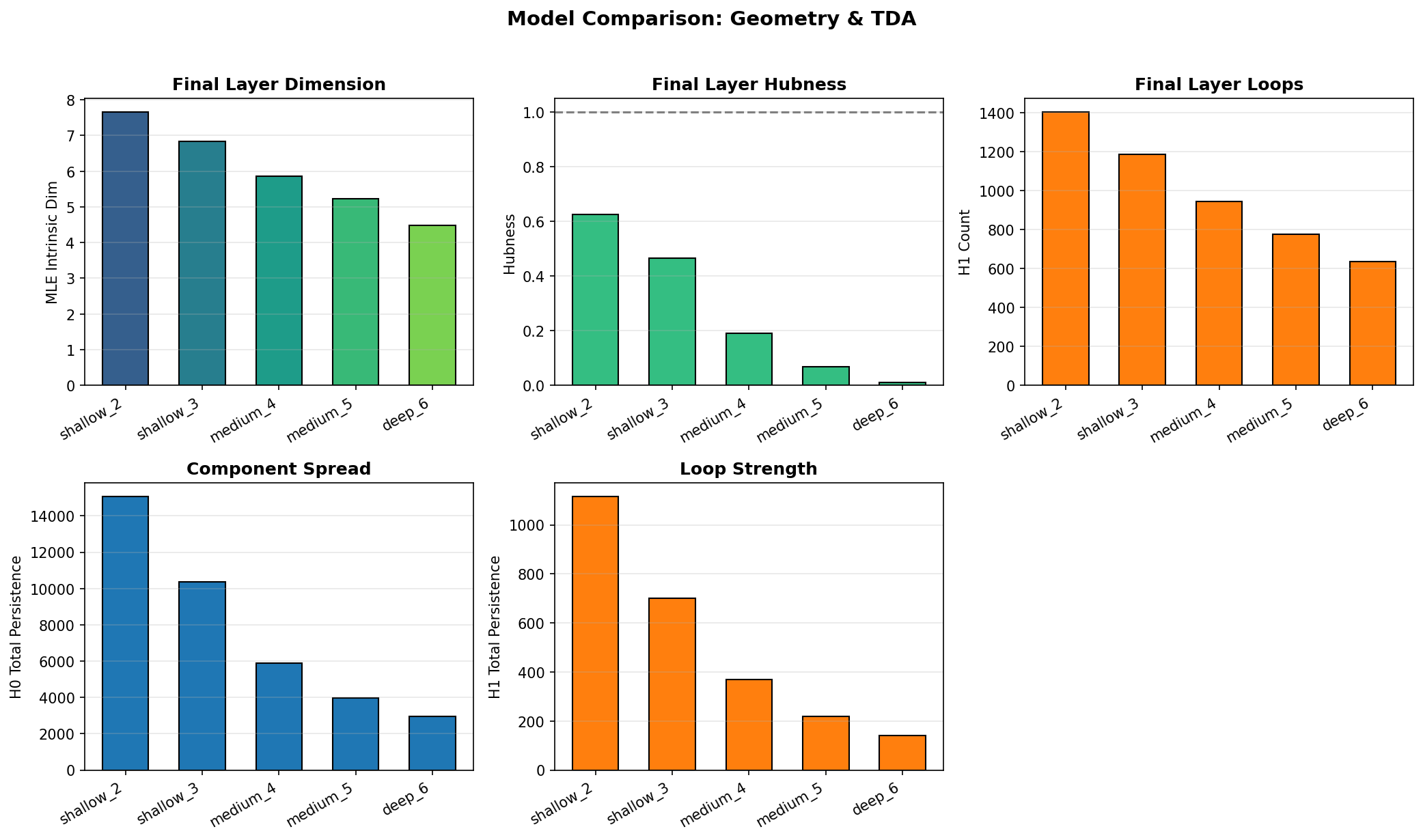
Comparing across depths reveals a consistent pattern: deeper networks compress more aggressively. The 2-layer network ends with intrinsic dimension around 7.7; the 6-layer network compresses to 4.5. Hubness drops toward zero in deeper networks, and both H0 and H1 persistence decrease with depth. More layers means more opportunity to simplify the representation geometry.
This contrasts sharply with the expansion patterns of transformers. Where GPT-2 spreads representations outward as it processes tokens, MLPs compress them inward. Both are valid geometric strategies serving different computational goals: transformers accumulate context across tokens, while MLPs project inputs toward decision boundaries.
Scaling Up: 20,000 Samples
The initial transformer findings with 500 samples raised a question: would the patterns persist at scale, or were they artifacts of limited sampling? With 500 points, the Vietoris-Rips complex is computationally tractable, but statistical confidence is limited.
The latest version of ToDACoMM supports extraction of 10,000 to 50,000 activation samples from transformers, with intelligent subsampling for the TDA computation itself. The workflow: extract activations for all samples, characterize geometry (intrinsic dimension, hubness, distance distributions) on the full set, then subsample to 2,000 points for Ripser. This preserves the statistical benefits of large samples while keeping homology computation feasible.
The geometry characterization step, new in this version, computes several metrics before TDA:
- MLE intrinsic dimension: Maximum likelihood estimate of the manifold dimension
- Local PCA dimension: Average dimensionality of local neighborhoods
- Hubness score: Skewness of the k-occurrence distribution
- Distance statistics: Mean, variance, and distribution of k-NN distances
These metrics are cheaper to compute than persistent homology and provide complementary information. Intrinsic dimension tells us how many degrees of freedom the representations actually use; hubness indicates whether the space has pathological concentration; distance distributions reveal the spread and clustering of points.
GPT-2 at Scale: Compression Through Depth
Running GPT-2 (124M parameters) and GPT-2-medium (354M parameters) on 20,000 WikiText-2 samples revealed something I had suspected but not confirmed at smaller scales: the intrinsic dimension of representations compresses dramatically through the network.
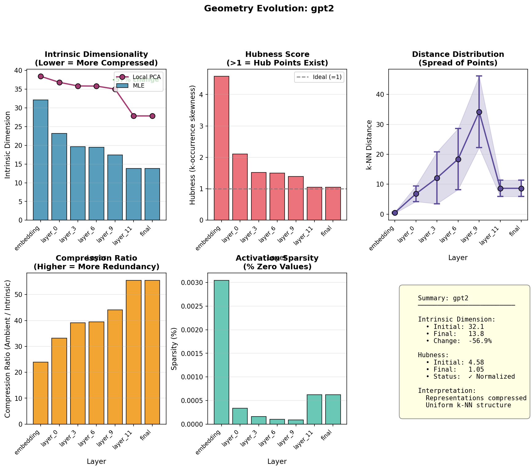
At the embedding layer, GPT-2's MLE intrinsic dimension is approximately 32. By the final layer, it drops to around 14, a 57% reduction. The model starts with high-dimensional token embeddings and progressively squeezes them into a lower-dimensional subspace as it builds contextual representations.
The hubness trajectory is equally striking. The embedding layer has hubness of 4.58, indicating severe hub structure; some token embeddings appear in many other tokens' nearest-neighbor lists. Through the layers, hubness drops monotonically, reaching 1.05 by the final layer. The network transforms pathologically concentrated embeddings into uniformly distributed representations.
The distance distribution reveals something unexpected: representations spread apart dramatically in middle layers (peaking at layer 9), then reconsolidate in final layers. The mean k-NN distance rises from 0.48 at embedding to 34.2 at layer 9, then falls to 8.6 at the final layer. This expansion-then-contraction pattern suggests the network first separates representations to build context-specific meanings, then gathers them back for prediction.
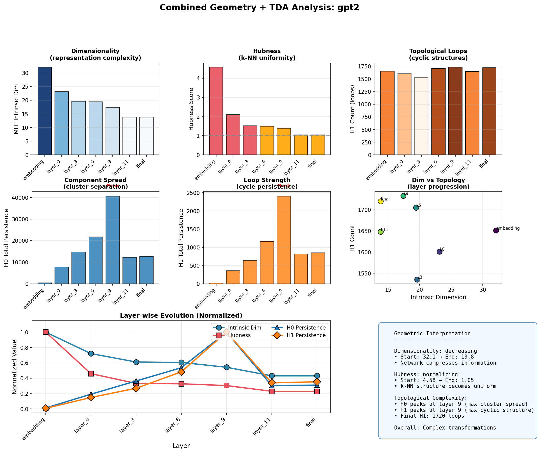
The TDA metrics corroborate this picture. H0 total persistence (cluster spread) peaks at layer 9, matching the distance distribution peak. H1 count (loop structures) remains relatively stable at around 1,700 across all layers, suggesting the cyclic structure is inherent to the representation manifold rather than an artifact of particular layers. The "Dim vs Topology" scatter plot shows the progression: embedding starts high-dimensional with moderate loops, middle layers spread out in both dimensions, and final layers compress dimensionally while maintaining topological structure.
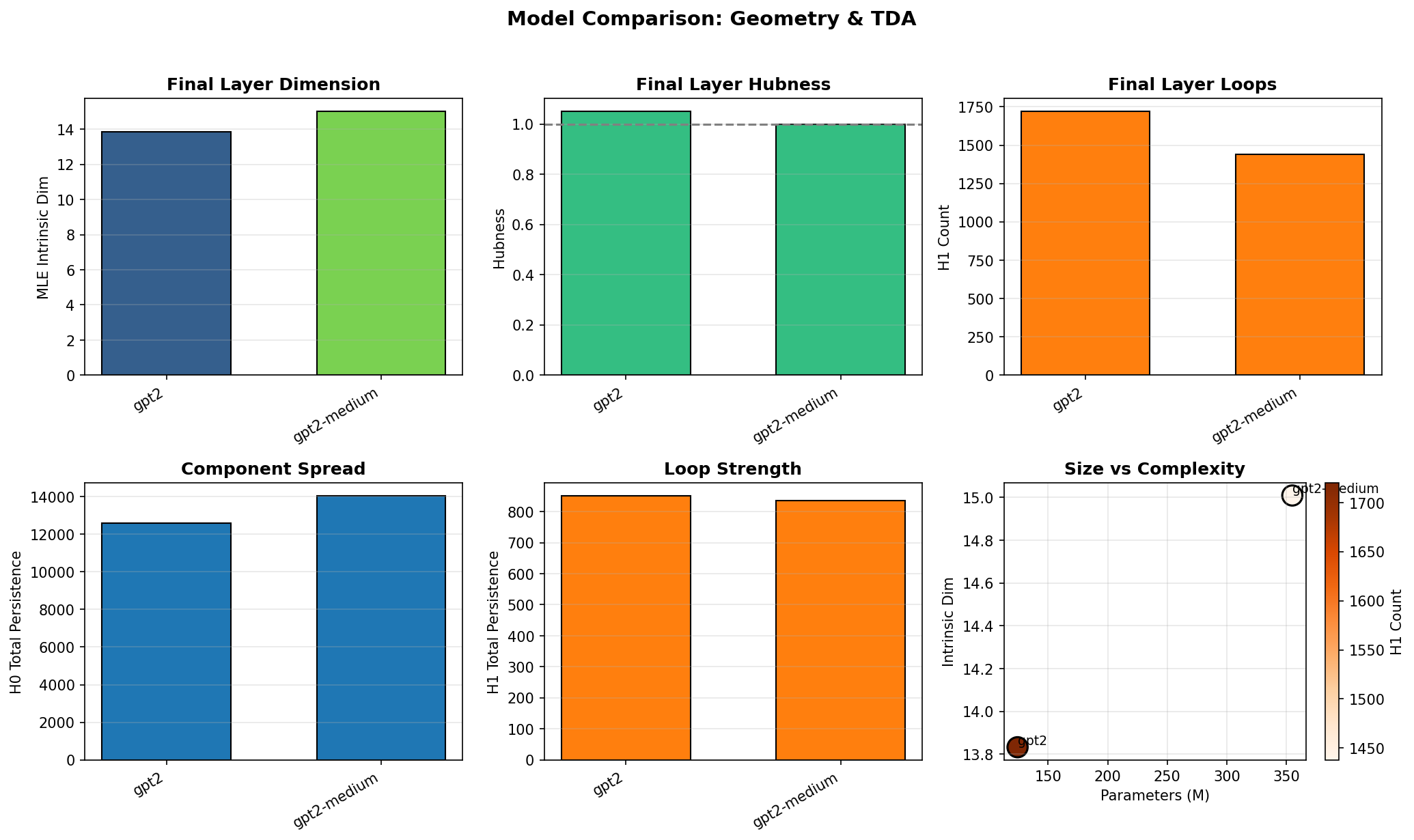
Comparing GPT-2 to GPT-2-medium reveals scaling effects. The larger model maintains slightly higher intrinsic dimension (15.0 vs 13.8) and achieves near-perfect hubness normalization (1.0 vs 1.05). Interestingly, GPT-2-medium has fewer H1 loops (1,438 vs 1,720) despite having nearly 3x the parameters. More capacity may enable simpler topological structure; the larger model can represent the same information with less geometric complexity.
SmolLM: A Different Architecture, A Different Trajectory
SmolLM presents a contrast to GPT-2. Where GPT-2 has 12 layers with 768-dimensional hidden states, SmolLM-135M has 30 layers with 576-dimensional hidden states. More layers, smaller width. Running the same 20,000-sample analysis reveals a fundamentally different geometric trajectory.
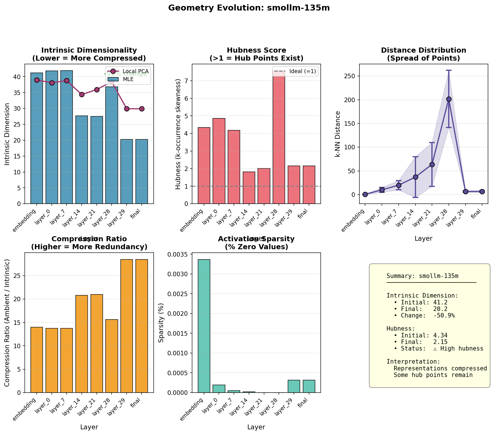
The intrinsic dimension trajectory shows two distinct phases. In layers 0-7, dimension remains high around 43, essentially unchanged from the embedding. Then a sharp transition occurs: by layer 14, dimension drops to 27, where it plateaus through layer 21. This is not the smooth, monotonic compression of GPT-2; it is a phase transition, a discrete jump in the representation regime.
The penultimate layer anomaly is the most striking feature. Layer 28 shows hubness spiking to 7.81, far above any other layer. The k-NN distance distribution explodes, with mean distance reaching 204 (compared to 64 at layer 21). Something dramatic happens in the penultimate layer: representations spread apart explosively, creating severe hub structure, before the final layer re-normalizes them.
What could cause this? One possibility: the penultimate layer is creating maximally separated "hub" representations to give the final layer clean inputs for prediction. Another: the architecture's depth-to-width ratio creates bottlenecks that manifest as geometric instability near the output. The pattern is reproducible; SmolLM-360M shows the same penultimate spike at layer 24, though attenuated (hubness 3.33, distance 156).
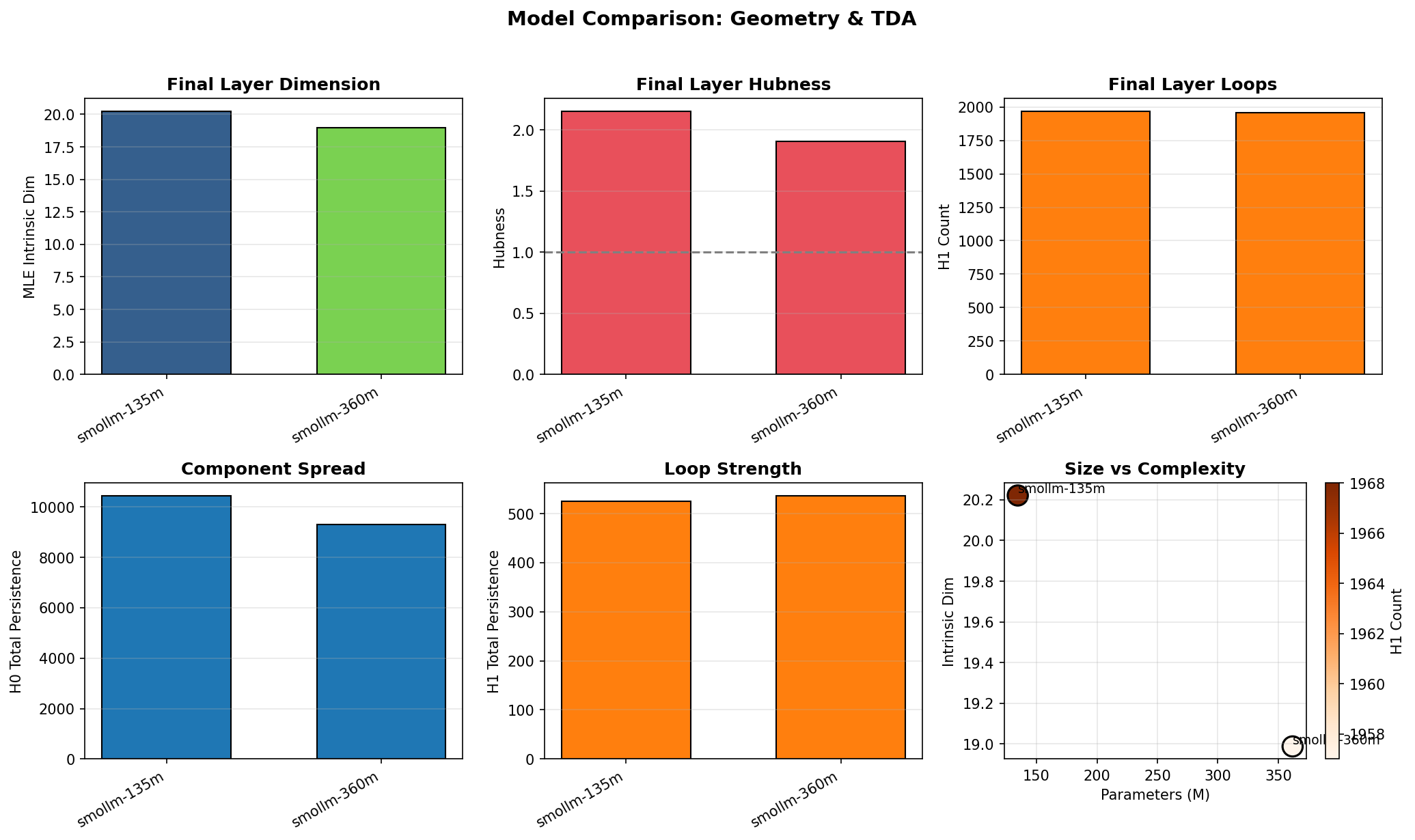
Comparing SmolLM to GPT-2 at similar parameter counts reveals architectural fingerprints:
| Model | Params | Layers | Final Dim | Final Hubness | H1 Count |
|---|---|---|---|---|---|
| GPT-2 | 124M | 12 | 13.8 | 1.05 | 1,720 |
| SmolLM-135M | 135M | 30 | 20.1 | 1.99 | 1,969 |
| GPT-2-medium | 355M | 24 | 15.0 | 1.00 | 1,438 |
| SmolLM-360M | 362M | 32 | 19.1 | 1.87 | 2,051 |
SmolLM retains higher intrinsic dimension (20 vs 14), maintains higher hubness (~2 vs ~1), and builds more topological loops (~2,000 vs 1,400-1,700). The deeper, narrower architecture preserves more structure through to the final layer. Whether this is beneficial depends on the task; more structure means more information retained, but also more complexity to navigate during inference.
The two-phase compression and penultimate anomaly are SmolLM's topological signature. They distinguish it from GPT-2's smooth expansion-contraction as clearly as GPT-2's 95x expansion ratio distinguishes decoders from BERT's 2x.
The Encoder-Decoder Divide
BERT showed an expansion ratio of 2x. Representations in the final layer were only twice as spread as in the embedding layer.
GPT-2 showed 95x. Other decoders ranged from 55x (DistilGPT-2) to 694x (SmolLM2-360M).
| Model | Parameters | Expansion Ratio |
|---|---|---|
| BERT | 110M | 2x |
| DistilGPT-2 | 82M | 55x |
| GPT-2 | 117M | 95x |
| Pythia-70M | 70M | 143x |
| Pythia-410M | 410M | 189x |
| SmolLM2-135M | 135M | 298x |
| Qwen2-0.5B | 500M | 629x |
| SmolLM2-360M | 360M | 694x |
Why such a stark difference?
Consider what BERT and GPT-2 are doing differently. BERT uses bidirectional attention: every token attends to every other token from layer one. When processing "The cat sat on the mat", the representation of "cat" at layer 1 already incorporates information from "sat", "mat", and everything else. The full relational structure is available immediately.
GPT-2 uses causal attention: each token can only attend to preceding tokens. The representation of "cat" at layer 1 only knows about "The". By layer 6, it knows about "The cat sat on the". By the final layer, it has accumulated the full prefix. This progressive accumulation requires the representation to expand; each layer must encode more context than the last.
In geometric terms: BERT's representations don't need to unfold because all context is accessible from the start. GPT-2's representations must unfold progressively, encoding an expanding window of context into the geometry. The 2x versus 55-694x expansion ratios are the topological signature of this architectural difference.
Architecture Fingerprints
Within decoder families, topological signatures remained consistent across training variations. The three Qwen variants (2-0.5B, 2.5-0.5B, Coder-0.5B) showed expansion ratios of 629x, 673x, and 642x respectively. These models differ in training data (general vs code) and version, but their topological fingerprint is stable.
Pythia scaled with model size: 143x at 70M parameters, 189x at 410M. More parameters means more capacity to expand the representation space.
These are fingerprints. Architecture determines topological regime more than training recipe does. If you told me a model's expansion ratio, I could likely guess its architecture family.
SmolLM2 was anomalous, with expansion varying from 298x (135M) to 694x (360M). This might reflect architectural differences between sizes, or something about how this family encodes information. The variance is worth investigating.
Cyclic Structure
Every model showed non-trivial H1 at 500 samples. There are loops in the representation geometry of every transformer I examined.
What does H1 mean in deep learning terms? If representations trace out a circular path in activation space as you vary some property of the input, that's H1. The grokking model learned circles because modular arithmetic is cyclic. What circular structure might language models learn?
Possibilities: syntactic patterns that recur (subject-verb-object cycles), semantic fields with circular relationships (days of the week, compass directions), positional patterns from the periodic positional encodings. The H1 persistence might be detecting some of this learned periodicity.
SmolLM2-360M stood out: H1 total persistence of 129.52, more than 3x higher than the next model. This model builds unusually strong cyclic structure. I do not yet understand what this corresponds to in terms of learned features, but it distinguishes this model topologically.
Limitations
ToDACoMM is descriptive, not predictive. It measures representation geometry but does not explain why models behave as they do. The 55x expansion of DistilGPT-2, for example, coincides with best-in-class perplexity among decoders, but we know that correlation does not automatically imply causation and so we cannot claim that that is a causal relationship. However, ToDACoMM may reveal a few interesting directions for teams who want to build models, and who might use such findings as a way to steer the direction of their model's development.
Further, ten models across five families is enough to see some general patterns and form hypotheses. It is not enough to make strong claims about the mechanism of learning purely using topological methods or measures. From a data standpoint, WikiText-2 is one dataset, and our findings on the topology of learning in these models might differ on other datasets.
Another thing worth bearing in mind, is that persistent homology is a coarse invariant. Two spaces with identical $H_0$ and $H_1$ can differ in geometrically significant ways. We are measuring coarse-grained shape, and not fine structure.
The PCA projection discards information. Patterns in the discarded 5% of variance might matter. This is a pragmatic choice, not an ideal one.
While these are not reasons to dismiss the findings, they impose restrictions on what we can claim. ToDACoMM is, therefore, an empirical tool for characterization, not a full theory of representation learning.
The Shape of What Was Carved
Gradient descent on the loss landscape carves out a representation manifold. The topology of this manifold reflects both the optimization dynamics and the structure of the training data.
Encoders, with bidirectional attention, carve compact spaces; context is globally available, so representations don't need to expand to encode it. Decoders, with causal attention, carve expansive spaces; context must be accumulated layer by layer, and the accumulation manifests as geometric expansion.
The 2x versus 55-694x divide follows from attention's arrow. This isn't a mysterious emergent property; it's a direct consequence of what the architectures are computing.
Within the carved spaces, cyclic structures form. Whether these reflect the periodicity of language, learned positional structure, or something else, they are consistently present. The grokking paper showed that models can learn geometrically appropriate representations (circles for cyclic arithmetic). The H1 findings suggest language models also learn geometric structure that reflects their training data.
Poincaré connected topology and dynamics in the 19th century. Neural networks are a domain where this connection can be measured empirically.
Directions
The large-scale experiments with GPT-2 and the MLP baselines have answered some initial questions while opening new ones. The encoder-decoder divide persists at 20,000 samples; the expansion-then-contraction pattern in GPT-2's distance distributions is robust. But several threads remain:
-
Training dynamics: Track topological changes during training. Does grokking have a topological signature? When does the encoder-decoder divide emerge? The MLP training pipeline now makes this tractable; one could checkpoint activations at each epoch and watch the geometry evolve.
-
The expansion-contraction pattern: GPT-2's representations spread dramatically in middle layers then reconsolidate. SmolLM shows a different pattern: two-phase compression with a penultimate layer explosion. Is this a width-vs-depth tradeoff? Do wider models (GPT-2) smooth their trajectories while deeper, narrower models (SmolLM) accumulate instabilities?
-
The penultimate layer anomaly: SmolLM's layer 28 shows extreme hubness (7.58) and H0 persistence (253k), an order of magnitude above surrounding layers. This pattern is reproducible across SmolLM sizes. What computational purpose does this serve? Is it a bottleneck effect, a feature of the architecture, or something about how the model was trained?
-
MLP depth effects: Deeper MLPs show monotonically simpler final topology. Is there a critical depth beyond which additional layers provide diminishing topological simplification? The 6-layer preset approaches this question but does not answer it.
-
$H_1$ interpretation: The cyclic structures persist across model scales and architectures. What do they correspond to? The stability of H1 count across GPT-2's layers (around 1,700 throughout) suggests these cycles are fundamental to the representation manifold, not layer-specific artifacts.
-
Connection to weight dynamics: I've been exploring a complementary approach in Deep Learning Dynamics, which uses perturbation analysis and Lyapunov exponents to measure how neural network weights evolve during training. ToDACoMM measures what gets carved in activation space; Deep Learning Dynamics measures how the carving happens in weight space. The preliminary finding that transformers universally diverge in weight space while showing dramatic expansion ratios in activation space suggests these phenomena may be related. The new geometry characterization metrics (intrinsic dimension, hubness) provide additional handles for connecting the two perspectives.
The framework is open source. The methodology and statistical analysis are documented. Others can extend this to their own models and domains.
ToDACoMM is available on GitHub. The technical report includes methodology, bootstrap confidence intervals, and ablation studies.