Random Seeds and Training Trajectories
Every neural network training run begins with a random seed. A different seed means different initial weights, which means a different trajectory through the loss landscape, which may or may not arrive at the same destination.
I've been thinking about this for a while, in the context of understanding the relationship between dynamical systems and the internal workings of neural networks. The question: do small changes in initialization lead to similar or different final solutions? In other words, do deep learning models that are essentially learning from feedback loops and errors, subject to sensitive dependence upon the initial conditions of initialization of weights and biases?
Methodology
The methodology I developed to answer this question treats training as a dynamical system and asks: how sensitive is this system to its initial conditions? The approach borrows from Lyapunov's work on dynamical stability, a framework developed in the late 19th century to understand whether planetary orbits would remain stable or fly apart. This same analysis has been replicated and used numerous times in the late 20th century as numerous dynamical and chaotic systems came to be studied. I am certain that this stability analysis has also been performed on deep neural networks especially since there are so many labs interested in performing training with as low a resource footprint as possible, which in turn bring stability of training into the foreground.
The procedure I used here is straightforward. Initialize a model with a fixed seed. Create several copies with small Gaussian perturbations, typically 1% of each parameter's standard deviation, enough to nudge the weights without fundamentally changing them. Train each perturbed model independently on the same data. Record the weight vectors after each epoch. Project the high-dimensional trajectories to principal components. Measure how the trajectories spread or converge.
@dataclass
class LayerSnapshot:
    """Snapshot of a single layer's state at a point in time."""

    # Weight statistics
    weight_mean: float
    weight_std: float
    weight_min: float
    weight_max: float
    weight_norm: float

    # Gradient statistics (if available)
    grad_mean: Optional[float] = None
    grad_std: Optional[float] = None
    grad_norm: Optional[float] = None

    # Eigenvalue statistics for weight matrix
    weight_singular_values: Optional[np.ndarray] = None
What emerges is a picture of the optimization landscape, not as a static surface but as a flow field where trajectories either merge toward attractors or diverge toward distinct basins.
Stability Metrics
Four quantities capture most of what matters about training dynamics:
Convergence Ratio measures whether trajectories come together or spread apart. It's the ratio of final spread to initial spread in the projected weight space. Below 1.0, the models ended up closer than they started; they converged. Above 1.0, they diverged.
Lyapunov Exponent (λ) quantifies the exponential rate of this convergence or divergence:
Positive λ indicates chaotic dynamics where small perturbations grow exponentially, the signature of a system sensitive to initial conditions. Negative λ indicates stable dynamics where perturbations decay. The exponent tells you not just whether trajectories diverge, but how fast.
Early/Late Ratio reveals when divergence happens. A ratio above 1.0 suggests early divergence, where models quickly find different paths. Below 1.0 suggests late divergence, where they track together initially but separate as training progresses. This distinction matters for understanding whether instability is fundamental or emergent.
PCA Variance Explained indicates how structured the dynamics are. Higher values suggest trajectories follow a low-dimensional manifold; lower values suggest high-dimensional, less predictable evolution.
Results
I analyzed 21 neural network architectures across three families: 10 dense networks trained on the circles dataset, 5 CNNs on MNIST, and 6 transformers on SST-2 sentiment classification. Each architecture was trained with multiple perturbed initializations, and the trajectories were compared.
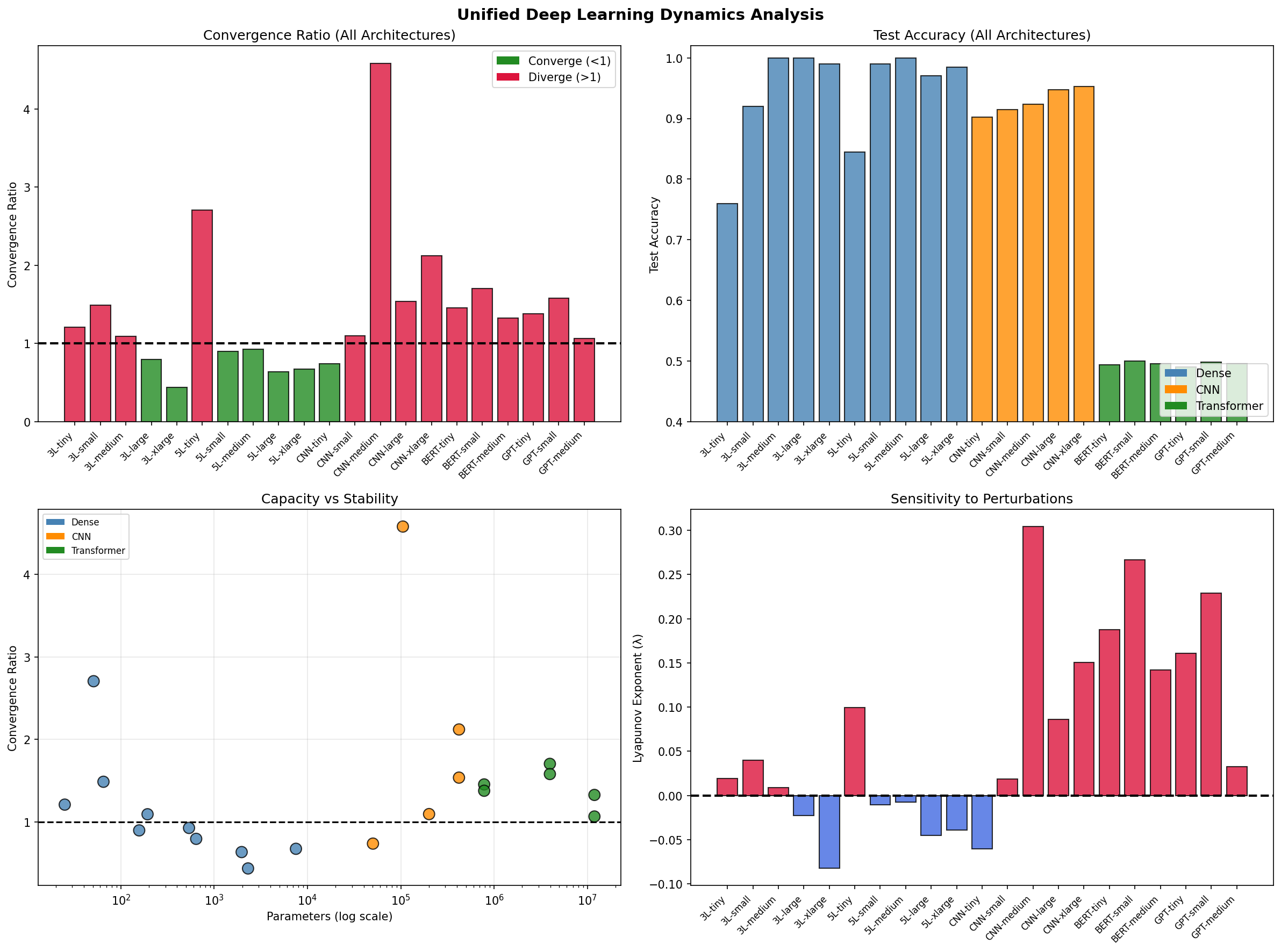
The master summary reveals stark differences: Dense networks cluster around convergence (ratio ≈ 1), while CNNs and transformers spread toward divergence.
The results were categorical:
| Family | Architectures | Convergent | Avg Ratio | Lyapunov λ |
|---|---|---|---|---|
| Dense | 10 | 6 (60%) | 1.09× | -0.004 |
| CNN | 5 | 1 (20%) | 2.01× | +0.100 |
| Transformer | 6 | 0 (0%) | 1.42× | +0.170 |
Dense networks are the most stable. Six of ten configurations converged, with an average spread ratio barely above unity. If you train a dense network twice with slightly different initializations, you'll often get very similar final weights. The Lyapunov exponent is negative; perturbations are dampened.
CNNs are substantially less stable. Only one of five configurations converged. The average spread ratio of 2.01× means perturbed models typically end up twice as far apart as they started. The convolutional structure, with its weight sharing and spatial hierarchies, admits multiple distinct solutions.
Transformers never converged. Zero out of six configurations. The attention mechanism creates a landscape where small initial differences cascade into large final differences. The Lyapunov exponent is the highest of all families.
Dense Networks
Within the dense family, larger networks tended toward convergence. The 3-layer XLarge configuration with 2,305 parameters converged with a ratio of 0.44×, the most stable architecture in the entire study. The 5-layer Tiny configuration with 51 parameters diverged at 2.71×, the least stable.
Depth had a nuanced effect. Shallower networks (3-layer) showed slightly more stable training than deeper ones (5-layer), with average convergence ratios of 1.01× versus 1.17×. This might seem counterintuitive; one might expect deeper networks to have more regularization through gradient flow constraints. But depth also means longer paths for perturbations to propagate.
class DynamicalSystemsAnalyzer:
    """
    Analyzes neural network training through the lens of dynamical systems.

    Treats the weight space as a phase space and training as a trajectory
    through this space, applying tools from nonlinear dynamics.
    """

    def __init__(
        self,
        tracker: DynamicsTracker,
        model: nn.Module,
        n_pca_components: int = 10,
    ):
        self.tracker = tracker
        self.model = model
        self.n_components = n_pca_components
The practical interpretation: for reproducible results on simple classification tasks, dense networks offer consistent behavior across seeds. For ensemble learning where you want diverse models, you might intentionally choose less stable configurations.
Transformers
Transformers presented a different picture entirely. No transformer configuration converged. BERT variants (bidirectional attention) showed average divergence of 1.50×. GPT variants (causal attention) showed 1.34×, slightly better but still divergent.
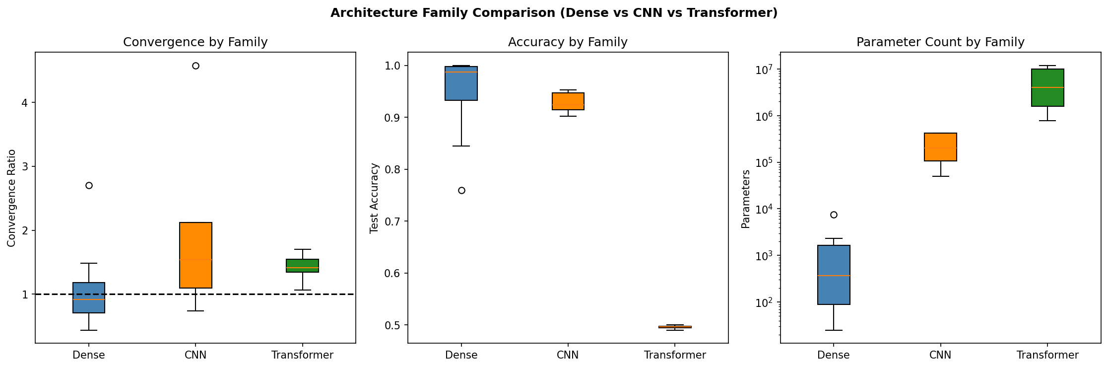
Box plots reveal that transformers, despite universal divergence, show tighter distributions than CNNs. The chaos is consistent.
The difference between BERT and GPT is interesting. One might expect bidirectional attention to be more stable, since each position has access to full context during training. But the data suggests otherwise. Causal masking in GPT apparently constrains the optimization landscape in ways that marginally improve stability, perhaps by reducing the degrees of freedom in gradient flow.
Larger transformers showed better convergence properties. GPT-medium with 12 million parameters achieved a ratio of 1.07×, while GPT-tiny with 780,000 parameters reached 1.38×. Overparameterization may provide smoother loss surfaces.
Trajectory Spread Over Training
Trajectory spread evolves differently across architectures:
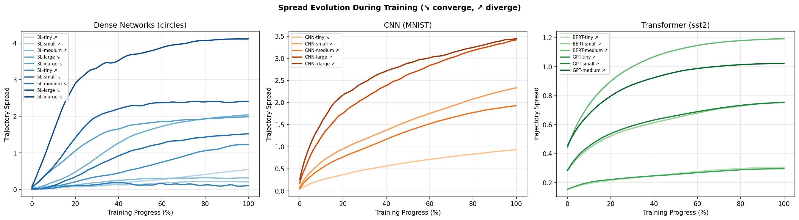
Spread evolution across families. Dense networks show falling curves (convergence); CNNs and transformers show rising curves (divergence).
Falling curves indicate convergent training, where perturbations are "forgotten" as training progresses. Rising curves indicate divergent training, where small initial differences amplify over time. The steepness of early changes suggests the initial learning phase is most sensitive.
Dense networks show predominantly falling curves. The optimization is pulling trajectories together. CNNs and transformers show predominantly rising curves. The optimization is pushing trajectories apart.
This has implications for checkpointing. If you're training a transformer and want to reduce initialization sensitivity, averaging checkpoints across different runs might help. The trajectories diverge, but early checkpoints before the divergence has compounded could be closer.
A Dynamical Systems Perspective
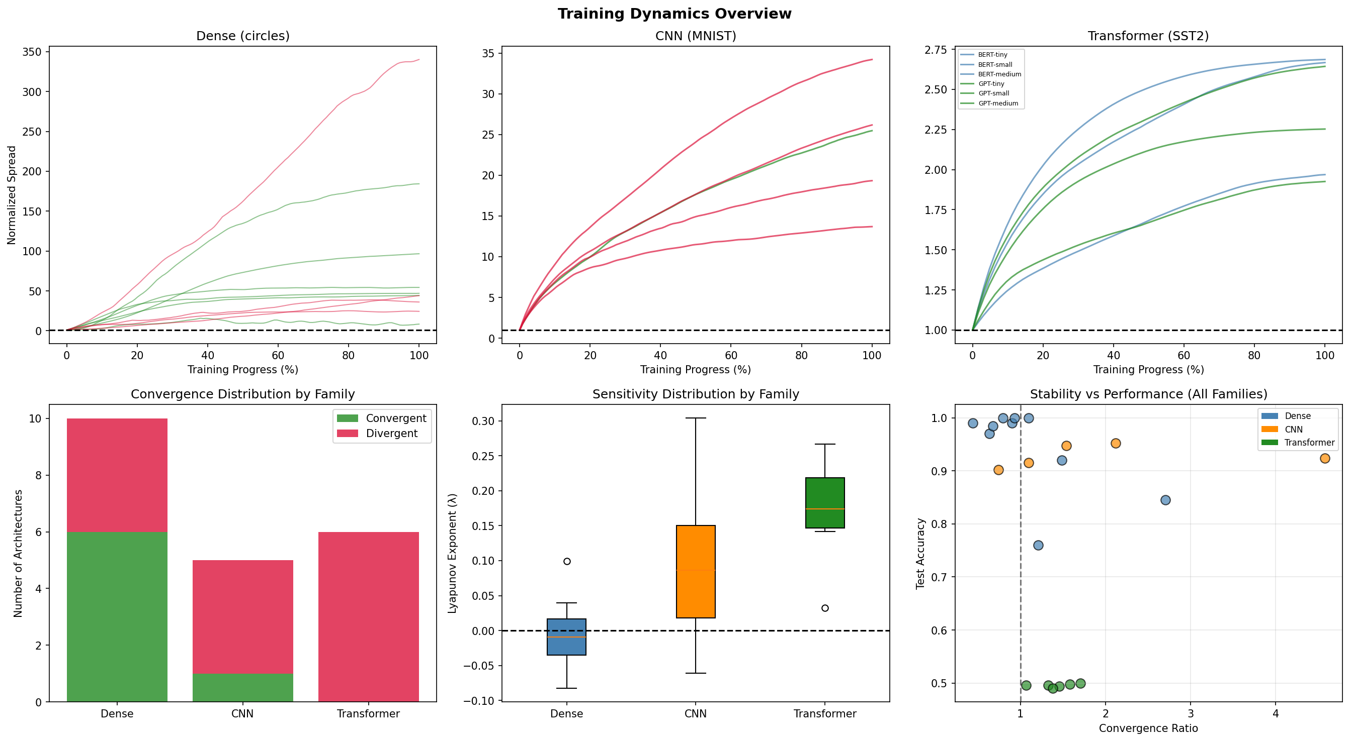
Cross-family dynamics comparison showing the full picture of convergence ratios, Lyapunov exponents, and accuracy distributions.
Applying dynamical systems theory to neural networks connects to older questions. Poincaré developed these tools to understand celestial mechanics, to predict whether the solar system would remain stable or eventually fly apart. The question was whether small perturbations, a slight change in Jupiter's position, would grow or decay over time.
Neural network training is a different system, but the same question applies. Small perturbations with a slight change in initial weights, grow or decay over epochs. The Lyapunov exponent here measures the sensitivity, just as it does for planetary orbits.
There is a distinc difference in the dynamics of neural networks and planetary orbits, however, as planetary orbits have continuous dynamics and training neural networks has discrete dynamics. Further, planetary systems are conservative; training has friction (weight decay) and injection (data). But the core insight transfers from one space to another, that some systems are stable, some are chaotic, and the architecture determines which ones pan out which way.
Practical Implications
For reproducibility: If you need consistent results across training runs, prefer dense architectures or accept that transformer training is inherently variable. Two transformer runs with different seeds will find different solutions. This isn't a failure of the training procedure; it's a property of the architecture.
For ensembles: The divergent architectures are your friends for ensemble diversity. Transformers naturally explore different solutions without needing special tricks. Dense networks may require more aggressive perturbation to achieve ensemble diversity.
For debugging: If a transformer training run fails, try a different seed before concluding the architecture is broken. The same configuration that fails with one initialization may succeed with another.
For architecture selection: Stability is a design consideration alongside accuracy and efficiency. For safety-critical applications where reproducibility matters, the extra stability of dense networks may outweigh their lower expressiveness.
What This Doesn't Tell Us
This analysis uses small-scale training, typically 10-50 epochs on reduced datasets. Production-scale training with billions of tokens might show different dynamics. The perturbation magnitude of 1% is somewhat arbitrary; different magnitudes might reveal different structure.
The metrics capture global properties of the trajectory ensemble but miss local structure. Two configurations with similar convergence ratios might have very different trajectory geometries.
And crucially: convergence or divergence says nothing about generalization and actual model performance. It is fair to say that the lyapunov exponents are not a good metric for generalization or model performance. A model that converges to the same weights every time might still overfit. A model that finds different solutions might find ones that generalize better. The dynamics describe the optimization, not the learned representation.
Connection to ToDACoMM
There's a natural connection to ToDACoMM, the project I built to measure the topology of trained representations using persistent homology. Deep Learning Dynamics measures how weights evolve during training; ToDACoMM measures what gets carved in activation space after training.
The preliminary observation is suggestive: transformers show both the most chaotic training dynamics (highest Lyapunov exponents, 0% convergence) and the most dramatic topological expansion (55-694× expansion ratios in activation space). Dense networks show both stable training and modest topological transformation.
Is this correlation causal? Do architectures with divergent weight trajectories necessarily produce topologically distinct representations? This remains an open question, one I'm continuing to investigate.
The Library: deep-lyapunov
The methodology described in this post has been packaged as deep-lyapunov, a Python library for analyzing neural network training stability. It's available on PyPI:
pip install deep-lyapunov
The library provides a clean API for stability analysis on any PyTorch model:
import torch.nn as nn
from deep_lyapunov import StabilityAnalyzer

# Your model
model = nn.Sequential(
    nn.Linear(784, 128),
    nn.ReLU(),
    nn.Linear(128, 10)
)

# Analyze stability
analyzer = StabilityAnalyzer(
    model=model,
    perturbation_scale=0.01,  # 1% perturbation
    n_trajectories=5,          # Compare 5 perturbed copies
)

results = analyzer.analyze(
    train_fn=your_training_function,
    train_loader=train_loader,
    n_epochs=10,
)

# Results
print(f"Convergence Ratio: {results.convergence_ratio:.2f}x")
print(f"Lyapunov Exponent: {results.lyapunov:.4f}")
print(f"Behavior: {results.behavior}")  # 'convergent' or 'divergent'

# Generate HTML report with embedded visualizations
results.save_report("stability_analysis/")
The library handles all the complexity: creating perturbed model copies, tracking weight trajectories during training, projecting to PCA space, computing Lyapunov exponents, and generating publication-ready reports.
For custom training loops, there's a manual recording mode:
analyzer = StabilityAnalyzer(model)
analyzer.start_recording()

for epoch in range(10):
    train_one_epoch(model, train_loader)
    analyzer.record_checkpoint()

results = analyzer.compute_metrics()
Logging is built in for visibility into what's happening:
import logging
logging.basicConfig(level=logging.INFO)
# Shows: Starting stability analysis, Training trajectory 1/5, Analysis complete...
The library is available at github.com/aiexplorations/deep-lyapunov and pypi.org/project/deep-lyapunov.
The Research Code
The full experimental pipeline used for the analysis in this post is also open source:
# Clone and install
git clone https://github.com/aiexplorations/deep_learning_dynamics
cd deep_learning_dynamics
pip install -e .[dev]

# Run full analysis
python -m experiments.unified_pipeline --output outputs/analysis

# Quick test
python -m experiments.unified_pipeline --quick

# Specific families only
python -m experiments.unified_pipeline --transformer-only
The output includes comprehensive reports, visualizations, and machine-readable metrics for all architectures analyzed.
Looking Forward
Several directions seem worth pursuing:
Scale: How do dynamics change with model size? Do larger transformers become more or less chaotic? The preliminary evidence suggests larger models are more stable, but this needs verification at scale.
Training recipes: Do learning rate schedules, warmup, or optimizer choices affect convergence? Can we engineer stability into otherwise divergent architectures?
Checkpointing: Can we identify stable checkpoints where perturbation sensitivity is lowest? This could inform checkpoint selection for production deployment.
Cross-architecture: Train the same task with dense, CNN, and transformer architectures. Compare not just final accuracy but trajectory stability. Understand the tradeoff.
The dice we roll when we pick a random seed matter more for some architectures than others. Understanding when and why is part of understanding what neural networks actually do.
The deep-lyapunov library is available on PyPI (pip install deep-lyapunov) and GitHub. The research code and experimental pipeline are available at deep_learning_dynamics.