I spent the last few months building Vajra BM25, a search engine that uses category theory as its organizing principle, and also delivers the current fastest BM25 search with Python, as of December 2025. The name "Vajra" comes from the Sanskrit word for "thunderbolt" or "diamond," and the project began as an experiment: could mathematical abstractions from category theory make a search engine's code cleaner without sacrificing performance?

The interesting thing when I went down this category theory rabbit hole, was that the category theory framing produced cleaner code and neat abstractions, and introduced me to a cool way of thinking about search. The resulting search engine also became remarkably fast over time. Initially, I was captivated by the elegance of using the category theory framing, but as time progressed, I realized that this could be built into a competent search engine as well, and leveraged some of the best scientific Python packages, vectorization, SIMD, and other optimizations to deliver three minor releases of Vajra search. It has been a very satisfying journey! The project started off as an innocent way to think of category theory abstractions to represent graph search. As I was working with text based search at work (Elastic) a lot, I realized that this could also be attempted. And here we are!

The latest benchmarks show Vajra achieving 180,000 to 800,000 queries per second, outperforming industry-standard engines like Tantivy (Rust) and Pyserini (Lucene) by orders of magnitude. This post documents what I learned along the way, including comprehensive benchmarks across six BM25 implementations and four datasets. But first, let me share how search engines work, because understanding the fundamentals made all the difference in building something fast.

The Anatomy of a Search Engine

At its core, every text search engine solves the same problem: given a query, find the most relevant documents from a corpus of documents. The solution has three fundamental components that I came to appreciate deeply while building Vajra.

1. The Index

The index is the data structure that actually makes search fast. Without an index, you'd have to scan every document for every query, which becomes impossibly slow for large corpora, and in computational complexity terms, is $O(nm)$ where n is the number of documents and m is the number of queries. Indexing solves this by reducing the complexity to $O(n+m)$ by using a data structure that allows for efficient retrieval of documents that contain a given term. There are two ways to think about indexing:

Forward Index (document → terms):

doc_1 → ["machine", "learning", "algorithms"]
doc_2 → ["deep", "learning", "neural", "networks"]
doc_3 → ["machine", "learning", "neural", "networks"]

Inverted Index (term → documents):

"machine"   → [doc_1, doc_3]
"learning"  → [doc_1, doc_2, doc_3]
"neural"    → [doc_2, doc_3]
"networks"  → [doc_2, doc_3]
"algorithms"→ [doc_1]
"deep"      → [doc_2]

The inverted index is the key tool of efficiency in most search engines. Instead of asking "what terms are in this document?", we ask "which documents contain this term?". For a query like "neural networks", we instantly get the candidate set {doc_2, doc_3} without scanning all documents. This inversion of perspective, I later realized, has a natural categorical interpretation.

2. The Scorer

Now that we have candidate documents, we need to rank them by relevance. BM25 (Best Match 25) is the dominant scoring function, developed in the 1990s and still used by Elasticsearch, Solr, and most modern search engines.

BM25 scores each document based on three factors: how often the query term appears in the document (term frequency), how rare the term is across all documents (inverse document frequency), and a normalization factor for document length. The formula balances these with tunable parameters k1 and b.

What struck me while implementing BM25 in Vajra is that scoring is fundamentally a morphism, a mathematical arrow from the product of query and document to a real number. This isn't just notation; it clarifies what the scorer does and how it composes with other operations. In category theory, a morphism is a function that preserves the structure of the category. In this case, the structure is the product of query and document, and the real number is the score.

This allows us to organize the code of our search engine in terms of the category theory abstractions we see here. And that gives us the potential to reuse these abstractions to build a different kind of mutable search pipeline. The scoring, then, is one of the steps of this pipeline.

3. The Ranker

With scores computed, the final step is returning the top-k results. This seems trivial, but at scale it matters: sorting a million scores is $O(n log n)$, while finding just the top 10 is O(n) with a partial sort. Small optimizations here compound quickly.

The Search Engine Landscape

In the process of building Vajra Search, as especially as I gravitated from graph search like BFS and DFS, which are common algorithms, I had the opportunity to explore some giants of the search engine landscape.

Lucene: The Industry Foundation

Apache Lucene (2000) is arguably the foundation of modern enterprise search. Written in Java, it powers Elasticsearch, Solr, and countless enterprise systems. Lucene's architecture reflects 25 years of production optimization:

flowchart LR
    subgraph LUCENE["Lucene Architecture"]
        direction TB
        S1[Segment 1] --> merge[Merge + Compact]
        S2[Segment 2] --> merge
        S3[Segment 3] --> merge
        merge --> disk[(Disk Storage)]
    end

    LUCENE --> F1[Disk-based indexes]
    LUCENE --> F2[Concurrent reads/writes]
    LUCENE --> F3[Near real-time search]

Lucene is designed for production durability: indexes persist to disk, support concurrent updates, and are able to scale horizontally via sharding. The trade-off is complexity and JVM overhead. Pyserini wraps Lucene via the Anserini toolkit, providing a Python API that can help us build with these capabilities in native Python applications (but with JVM dependencies nevertheless).

Tantivy: Lucene in Rust

Tantivy (2016) reimplements Lucene's architecture in Rust, gaining memory safety and roughly 2x performance over Java. It maintains the segment-based, disk-first design:

flowchart TB
    T[Tantivy] --> A[Segment Architecture]
    T --> B[Native Rust]
    T --> C[SIMD Postings]
    T --> D[Memory-mapped I/O]
    A --> E[Same design as Lucene]
    B --> F[No GC pauses]

Tantivy excels for applications needing persistent, updatable indexes with Rust's performance. However, the disk-based design adds I/O latency for pure query workloads. At some point, disk I/O is something Vajra is going to deal with. For the time being, I have preferred building indexes in memory. There is some caching possible within Vajra and in this sense, it is inspired by what Tantivy is able to do. Tantivy is super fast and performant given that it does this with disk I/O.

Rank-bm25: The Python Baseline

Rank-bm25 (2018) is the simplest BM25 implementation, a single Python file that's easy to understand:

class BM25Okapi:
    def __init__(self, corpus):
        self.corpus_size = len(corpus)
        self.doc_freqs = []  # Forward index: doc → term frequencies
        self.idf = {}        # Precomputed IDF values

    def get_scores(self, query):
        scores = np.zeros(self.corpus_size)
        for term in query:
            # Score ALL documents for this term
            for doc_idx in range(self.corpus_size):
                scores[doc_idx] += self._score_term(term, doc_idx)
        return scores

Rank-BM25 was my starting point to understanding the typical Python BM25 implementation meant for small tasks, and which is also not meant to be memory efficient, or fast. Indexing even smallish corpuses takes minutes, and it works in-memory. This is a tool for a limited job. The problem is clear: rank-bm25 uses a forward index and scores every document for every query. With a million documents and five query terms, that's five million score computations per query. While it not a great use of memory or compute, Rank-BM25 does get the job done and is simple for some of the smaller projects you may be building. It does not have complex abstractions like Vajra or ace engineering like BM25S, Tantivy or Lucene.

BM25S: Leveraging Eager Scoring

BM25S (2024) introduced a paradigm shift that I found elegant: eager scoring. Instead of computing scores at query time, pre-compute everything at index time:

flowchart LR
    subgraph INDEX["INDEX TIME - Slow, Once"]
        I1[Each term t] --> I2[Each doc d]
        I2 --> I3[Compute BM25 score]
        I3 --> I4[Store in sparse matrix]
    end

    INDEX -->|Pre-computed| QUERY

    subgraph QUERY["QUERY TIME - Fast, Many"]
        Q1[Look up term IDs] --> Q2[Slice matrix]
        Q2 --> Q3[Sum columns]
        Q3 --> Q4[Return top-k]
    end

The sparse score matrix stores pre-computed BM25 scores for every term-document pair:

So, what happens when you supply a query? Query time operations shrink to just sparse matrix slicing and addition. There are no IDF lookups, no BM25 formula evaluation, and none of the heavy lifting. This achieves 100-500x speedup over rank-bm25. The trade-off is memory footprint and no query-time flexibility. So, BM25S is a great tool for the job, and is probably a good starting point for building a search engine. I enjoyed benchmarking against it as I built Vajra search and the BM25S paper made for good reading and provided ideas and hints as to eager scoring, a technique which Vajra borrows from BM25S, in its own way.

Building Vajra: A Different Path

When I started Vajra, I wanted to combine ideas from different paradigms while using category theory to think about and organize the code. Having learnt about some of the aspects of category theory, I realized that this was a kind of scaffolding for other mathematics to be defined and built, and does not provide any differentiating capability in and of itself. So my approach was to use category theory to reframe the way we think about search.

We have discussed above how we need to compute inverted indexes, inverse document frequency, and perform BM25 computation and top-k sorting. These things don't change from implementation to implementation, and Vajra is no different in implementing these also in its pipeline, since after all, it too is a BM25 search engine. However the way these are implemented allows a kind of lazy computation and caching that is not implemented in other frameworks. Let's see more below.

flowchart TB
    subgraph INDEX["INDEX TIME"]
        I1[Build inverted index] --> I2[Precompute IDF]
        I2 --> I3[Sparse term-doc matrix]
    end

    INDEX --> Q1

    subgraph QUERY["QUERY TIME"]
        Q1{Cache check} -->|HIT| R[Return cached]
        Q1 -->|MISS| Q2[Get candidates ~1%]
        Q2 --> Q3[Vectorized BM25]
        Q3 --> Q4[Top-k sort]
        Q4 --> Q5[Cache result]
    end

    Q3 -.->|Key: Filter then score| Q3

Let's take a look at how Vajra's BM25 flow actually works, through this flow diagram. We will review different individual aspects of Vajra in this context below as well.

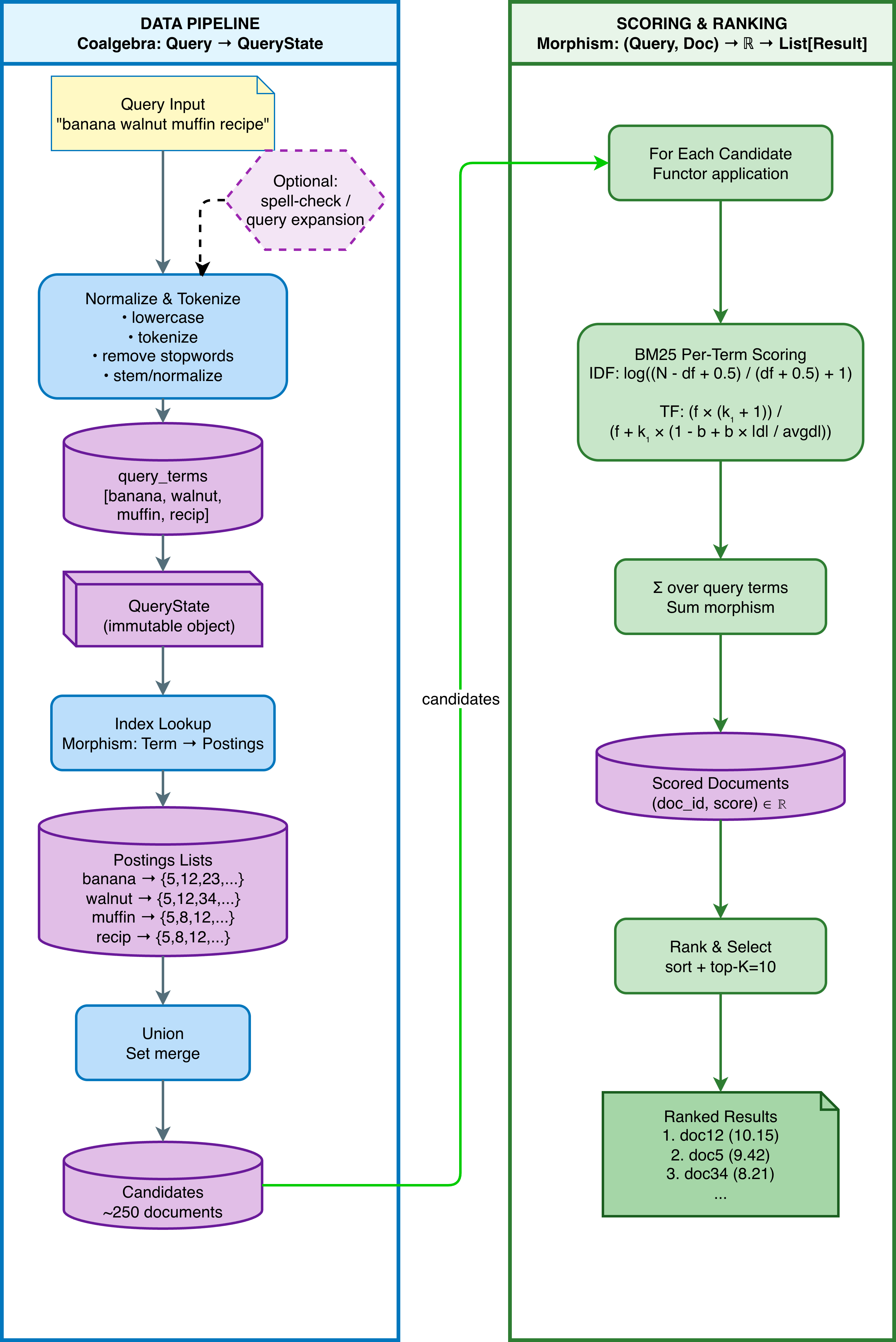
The insight that made Vajra fast came from thinking about what operations actually matter for speed and performance.

1. Inverted index filtering: For a query with three terms, only about 1% of documents contain all terms. Why score 500,000 documents when you can score 5,000?

2. LRU query caching: Real workloads have repeated queries. After the first execution, results are cached; subsequent calls return in nanoseconds.

3. Vectorized scoring: NumPy's SIMD operations score thousands of candidates in a single vectorized operation.

4. Lazy computation: Unlike BM25S, Vajra computes scores on-demand. This uses less memory and allows query-time flexibility.

The category theory framing, morphisms for scoring, coalgebras for search unfolding, provides the code organization. This allows me to build an interesting and different framework that may be composable and could provide a base on top of which to experiment in future. Having said that, the performance comes from these engineering choices, not from mathematical abstraction. Category theory, after all, provides a scaffolding on top of which other mathematical principles and ideas (such as those behind search) can be organized.

The Category Theory Foundation

As I have said earlier, I realized early on in this project, that category theory in and of itself cannot provide performance and search improvement techniques and abstractions of its own that can render pure speed. Therefore, category theory did not on its own make Vajra fast. The speed comes from NumPy, sparse matrices, and aggressive caching - these are essentially engineering choices. If you stripped out every morphism and coalgebra and kept only the vectorized scoring code, you would still get the same kind of performance, more or less.

So why use category theory at all? Because it gave me a clean way to organize the code. Let me show you what I mean with concrete examples.

How the Abstractions Organize Code

The codebase has a categorical/ module with three base abstractions: Morphism, Functor, and Coalgebra. Each provides an interface that derived classes implement.

Morphisms define composable transformations. The base class enforces an apply() method and provides composition via the >> operator:

class Morphism(ABC, Generic[A, B]):
    @abstractmethod
    def apply(self, a: A) -> B: ...

    def __rshift__(self, other: 'Morphism[B, C]') -> 'Morphism[A, C]':
        return ComposedMorphism(self, other)

This lets you build pipelines like where each step is a morphism with clear input and output types. The BM25 scorer becomes a morphism (Query, Document) → ℝ, which forces you to think about exactly what data flows in and out. Let is dig in a little.

Let's say we want to build a pipeline that preprocesses a query, tokenizes it, and then scores it. We can do this by composing the following morphisms:

preprocess >> tokenize >> score

This is a pipeline that preprocesses a query, tokenizes it, and then scores it. The preprocess morphism is responsible for preprocessing the query, the tokenize morphism is responsible for tokenizing the query, and the score morphism is responsible for scoring the query. This provides in practice a neat way to organize the code and to make it more readable and maintainable.

Coalgebras capture the "unfolding" pattern. In a nutshell, an unfolding is a way to represent a data structure as a tree. The base class requires a structure_map() method that takes a state and produces its successors:

class Coalgebra(ABC, Generic[X, FX]):
    @abstractmethod
    def structure_map(self, state: X) -> FX: ...

From this, I derived SearchCoalgebra, TreeSearchCoalgebra, and ConditionalCoalgebra. Search Coalgebras are a way to represent a search as a tree, and are used to represent the search space. Tree Search Coalgebras are a way to represent a search as a tree, and are used to represent the search space. Conditional Coalgebras are a way to represent a search as a tree, and are used to represent the search space. The BM25 search implementation extends Coalgebra with the signature QueryState → List[SearchResult]:

class BM25SearchCoalgebra(Coalgebra[QueryState, List[SearchResult]]):
    def structure_map(self, state: QueryState) -> List[SearchResult]:
        candidates = self.index.get_candidates(state.query_terms)
        ranked = self.scorer.rank(state.query_terms, candidates)
        return [SearchResult(doc, score, rank) for ...]

The same interface works for graph search (BFS, DFS) and tree exploration but with different derived classes. I found this genuinely useful; once you implement structure_map(), you get unfold(), trajectory(), and other coalgebraic operations for free.

Functors in Vajra are abstractions that allow you to "lift" a transformation—such as a morphism—so it works over entire containers rather than just single values. This is captured in code via an interface: every Functor lets you map any morphism across the relevant structure. For example, the ListFunctor implements a fmap_morphism method that takes a morphism and returns a new morphism, which processes each element of a list independently and collects the results.

class ListFunctor(Functor[A, List[A]]):
    def fmap_morphism(self, f: Morphism[A, B]) -> Morphism[List[A], List[B]]:
        return FunctionMorphism(lambda xs: [f.apply(x) for x in xs])

In the context of search, this means you can write a morphism that operates on an individual query or document, then seamlessly apply it to a whole batch of queries or search candidates using ListFunctor, enabling vectorized or batch-style computation in places where search might branch or aggregate multiple possibilities. This makes the code for candidate generation, ranking, and batch query processing both concise and highly reusable. The same pattern applies to MaybeFunctor, which handles computations that may fail by encapsulating values that might be missing, allowing the rest of the pipeline to remain clean and compositional even in the presence of errors.

The benefits of Vajra's architectural choices

By adopting category-theoretic abstractions like morphisms, functors, and coalgebras, Vajra cleanly disentangles data types from transformations and search strategies:

• Morphisms provide a systematic way to build and compose pipelines with explicit input/output types
• Functors let you automatically “lift” these pipelines across collections or optional values for batch or robust computation
• Coalgebras encode the core search dynamics in a way that's generic across strategies (tree, graph, conditional) so new algorithms can plug into the same interface and instantly inherit useful unfolding and traversal methods

This architectural clarity made it straightforward to add new scorers or search strategies: each abstraction exposes focused extension points, so it’s always clear where to slot in new logic and which minimal methods need to be implemented for composability. The monoid homomorphism insight, that BM25 scores are additive across terms (score(q₁ + q₂) = score(q₁) + score(q₂)) is also interesting and has practical consequences: you can cache term-level scores and sum them at query time, or compute upper bounds on partial scores for early termination. The algebraic structure pointed at optimization opportunities.

Benchmarking Vajra

Building the abstractions isn't where it stops, and to build a useful software application, we have to look at what's out there, benchmark the tool we're building to see where it fits in, and what relative benefits it may offer to users. So, to validate Vajra's performance, I benchmarked against a few other implementations:

To be clear, these are all BM25 implementations. All implementations compute the same essential BM25 formula:

$$\text{BM25}(q, d) = \sum_{i=1}^{n} \text{IDF}(q_i) \cdot \frac{f(q_i, d) \cdot (k_1 + 1)}{f(q_i, d) + k_1 \cdot \left(1 - b + b \cdot \frac{|d|}{\text{avgdl}}\right)}$$

The differences are in __how_ they compute it, and when.

Benchmark Results

I spent a lot of time benchmarking the initial build of Vajra against Rank-BM25, and then began excluding it from my benchmarks because of how slow the latter was. I moved on to BM25S as the peer framework of choice that I was benchmarking against, and also began testing against Tantivy and Pyserini eventually. While the latter is exceptional in its recall performance, with excellent Recall\@10 and NDCG\@10 (which measure whether the right docs came up, and in the right order) BM25S and Vajra have ultimately be the more comparable frameworks.

You'll see that latency (cold) is comparable for most frameworks, but it is in the warm lookup that Vajra BM25 really shines! This is due to the design decisions I have explained above in Vajra's architecture. See the video below for a Vajra specific search demo. This is using Vajra CLI, which is a command line based search tool which you can point at a JSON, and have a fast search engine right in your terminal!

BEIR/SciFact (5,183 documents, 300 queries)

What surprised me here: Vajra is 1,540x faster than BM25S and 820x faster than Tantivy. Pyserini has the best recall and NDCG, but at significant latency cost.

BEIR/NFCorpus (3,633 documents, 323 queries)

Nutrition and medical information retrieval dataset.

Wikipedia/200K (200,000 documents, 500 queries)

Wikipedia/500K (500,000 documents, 500 queries)

At 500K documents, Vajra maintains 180,000 QPS while Tantivy drops to 39 QPS. The gap widens at scale.

Improving Vajra's Performance

Vajra search started off being about as fast as BM25 and was for a couple of months quite a lot slower than BM25S! Tantivy and Pyserini were not in the picture at that stage of the project. My initial thinking was to see if I could build on top of category theory abstractions and see how we could speed things up, but came to the realization quickly that I would have to resort to engineering best practices - caching, the use of filtering, scoring and the use of sparse matrixes. Let's review each of these improvements below. If you use Vajra, you'll see numba used quite a lot in Vajra and for good reason.

LRU Query Caching

This was the single biggest optimization. Real workloads have repeated queries, and caching complete results means subsequent calls return instantly:

@lru_cache(maxsize=10000)
def search(self, query: str, top_k: int = 10):
    # First call: compute BM25 scores
    # Subsequent calls: instant cache hit

Combine this with user preference based caches and you can make Vajra search very performant and fantastically usable for a use case where repeated queries will come through from the bulk of users but different in every case.

Candidate Filtering with Inverted Index

Instead of scoring all documents like BM25S does with its sparse matrix, Vajra uses the inverted index to identify only the documents that contain query terms:

Query: "machine learning algorithms"

Traditional (Rank-BM25 or similar): Score 500,000 documents = 500,000 computations
Vajra: Filter to ~5,000 candidates, score only those = 5,000 computations

A large part of building a performant system seems to be to not try to do everything at once, but stage it all out, so that limited resources can be used in the best possible way.

Vectorized Scoring

Once candidates are identified, scoring uses NumPy vectorization:

# Score all candidates in one vectorized operation
scores = idf_vector @ tf_matrix * normalization_factors

No point reinventing the wheel that Numpy already provides. Matrix operations are super fast thanks to CPython bindings in Numpy and while it may not be as scalable as pure C or Fortran, it provides a significant speed up.

Sparse Matrix Storage

For corpora over 10K documents, the term-document matrix is 99%+ zeros. SciPy's CSR format avoids storing and computing on those zeros. This is another example of not overdoing stuff in the quest for performance.

Partial Sort for Top-K

Instead of sorting all scores, np.argpartition provides $O(n)$ average complexity:

# O(n) partial sort instead of O(n log n) full sort
top_indices = np.argpartition(scores, -k)[-k:]

Note that none of the above are exotic mathematics even if category theory does inform the architecture of Vajra BM25. Most of it is sane engineering you would recognize as a senior engineer or architect, and would likely build into any other project which you want high performance in.

Understanding the Latency Numbers

I want to be transparent about what the benchmark numbers mean. The reported latencies (0.001-0.006ms) represent averages after warmup with caching. Here's what to expect in practice:

As of v0.3.0, if you're using the Vajra CLI with single queries ($ vajra-search -q "query"), each invocation creates a new engine with an empty cache. Expect ~0.5ms latency. In interactive mode, subsequent queries benefit from caching and approach the benchmark speeds. The CLI is a super easy way to see Vajra in action.

For library usage, keep the VajraSearchOptimized instance alive across queries to benefit from the LRU cache. After 10-20 queries, average latency drops to sub-0.01ms. This is a great way to use Vajra as a library in your own projects.

Why Are the Other Search Engines Slower?

Tantivy's performance was a surprise

Despite being written in Rust, which is a high performance compiled language, Tantivy is 4,000x slower than Vajra on large datasets. This kinda puzzled me at first, and then I found out more about Tantivy and what is is built for, and how.

1. Disk I/O: Tantivy's index is disk-based, adding I/O latency
2. No query caching: Each query recomputes from scratch, unlike Vajra which adopts an LRU cache
3. Python bridge: The tantivy-py bindings add overhead. Despite built in Rust, the Python bindings introduce another layer of abstraction as a wrapper. Short of testing everything in Rust, this is the only option I have to use Tantivy, though.
4. Different priorities: Tantivy optimizes for persistence and updates, not raw query speed. Vajra is built for speed and efficiency, even though it started off as an experiment in using mathematical abstractions to build search. As such, Vajra is not optimized for persistence and updates.

The Pyserini Trade-off

Pyserini (Lucene) has the best accuracy on BEIR datasets but comes with costs: 2,000x slower query latency, 5-10x slower build times, and requires Java 11+ runtime. For applications where ranking quality is paramount and latency isn't critical, Pyserini remains valuable.

Accuracy Analysis

Lucene is the foundation of superb search engines like Elasticsearch for a reason! I'm sure there is scope for improvement here. Vajra is great at low latency queries, but perhaps the accuracy of the results as measured by NDCG@10 and Recall@10 require further improvement. Vajra still manages a better overall performance than BM25S and Tantivy, althought it lags behind Pyserini, which adopts Lucene. Let's look at the metrics for BEIR based searches.

BEIR dataset searches:

Pyserini wins on BEIR accuracy by 1-2%. Vajra, as you can see, is competitive but not best-in-class. Now, let's look at Wikipedia searches and the accuracy performance thereof.

Wikipedia dataset searches:

On Wikipedia, Tantivy leads while Pyserini degrades significantly. Vajra sits in the middle, somewhat competitive but rarely best.

When to Use Each Engine

Benchmark Methodology

For reproducibility, here's how I ran the benchmarks:

Hardware

Process

The benchmark script follows this sequence for each engine:

1. Load Dataset: BEIR datasets from HuggingFace; Wikipedia from pre-downloaded JSONL
2. Check Index Cache: Compute corpus hash, look for cached index
3. Build Index (if not cached): Each engine has its own indexing logic
4. Save Index to Cache: Pickle indexes for subsequent runs
5. Batch Query Evaluation (cold cache): Run all queries as a batch
6. Single Query Evaluation (warm cache): Run each query individually, compute metrics

Index Caching

I used persistent index caching to avoid expensive rebuilds:

For Vajra on 500K documents, index build takes about 16 minutes. With caching, subsequent runs load in under 5 seconds.

Running the Benchmarks Yourself

Start with a new Python environment and execute the following bash commands:

# Clone the repository to get the benchmarking scripts
git clone https://github.com/aiexplorations/vajra_bm25.git
cd vajra_bm25

# (Optional) Create a virtual environment here if you prefer isolation
# python -m venv .venv
# source .venv/bin/activate

# Install dependencies
pip install vajra-bm25[optimized] rank-bm25 bm25s beir rich tantivy
# doing a pip install is needed to have the whl in your environment

# Optional: Pyserini (requires Java 11+)
pip install pyserini

# Benchmark script is present only in the repo, does not ship with the whl file.
# Run BEIR benchmarks
python benchmarks/benchmark.py --datasets beir-scifact beir-nfcorpus

# Run Wikipedia benchmarks
python benchmarks/benchmark.py --datasets wiki-200k wiki-500k

# Force rebuild (ignore cache)
python benchmarks/benchmark.py --datasets wiki-200k --no-cache

Using Vajra Search

If you have read this far and have tried out Vajra BM25 in the CLI or as a package, thank you! You can use Vajra for any latency-intensive or performance-intensive Python specific workload, and I would love to hear about how you are using it if you are.

For starters, since I have built Praval earlier, I want to integrate Vajra BM25 into it. I have already built a CLI for Vajra BM25 and want to use it in Praval. One of the cool use cases I see for Vajra is in enabling agents to quickly search code bases, or datasets, or text corpuses. This can become a game changer for large scale multi-agent systems.

Closing Thoughts

Building Vajra taught me that the fastest solution often comes from questioning assumptions. Everyone knew that sparse matrix multiplication was the fast way to do BM25 (thanks to BM25S). But I found that filtering candidates first, then scoring only those, combined with aggressive caching, could be even faster.

The category theory framing was a useful thinking tool, even if it doesn't directly contribute to performance. Clearly separating concerns within the code base makes the application neat and maintanable. It helped me see search as a general pattern, morphisms mapping queries to scores, coalgebras unfolding search states into results. Whether that abstraction is worth the learning curve is a question each developer has to answer for themselves.

For most applications, Vajra offers a good trade-off: competitive accuracy with dominant speed. The code is available if you want to try it or build on it, or build other open source applications.

Links and References:

• Vajra BM25 Repo: github.com/aiexplorations/vajra_bm25
• Vajra BM25 on PyPI: pypi.org/project/vajra-bm25
• Vajra BM25 Benchmark docs: docs/vajra_benchmark_comparison.md
• Category Theory for Programmers: Bartosz Milewski
• Pyserini
• BM25S:
• Tantivy
• Rank-BM25
• Praval
• BEIR
• Wikipedia
• JSONL
• LRU Cache
• Partial Sort